¿Podemos Hacer Fine-tuning de un Modelo de 70B en una Sola GPU?
En los dos artículos anteriores we attacked the cost of fine-tuning from two angles. Full fine-tuning (article 2) showed that an AdamW ejecución de entrenamiento needs roughly 16 bytes per parameter — a 7-billion-parameter model demands about 112 GB of memoria de GPU, already exceeding a single A100's 80 GB capacity. LoRA (article 3) dramáticamente reduced the trainable parameter count by decomposing actualización de pesoss into low-rank matrices, slashing optimizer-state memory from tens of gigabytes to mere megabytes. Pero aquí está el problem LoRA didn't solve: the modelo base congelado still needs to fit in memoria de GPU.
With LoRA, a 7B model in FP16 still occupies about 14 GB for the base weights alone — manageable on a modern GPU. But what about a 70-billion-parameter model? In FP16, that's $70 \times 10^9 \times 2$ bytes $= 140$ GB just for the pesos congelados, before we add a single LoRA adapter or gradient buffer. No single consumer or even server-grade GPU can hold that. Full fine-tuning of 70B would need roughly $70 \times 10^9 \times 16 \approx 1.12$ TB — requiring a cluster of high-end GPUs with paralelismo de modelo.
Entonces la pregunta se convierte en: can we keep the base weights in a more compressed format? What if, instead of storing each frozen weight as a 16-bit float, we stored it as a 4-bit integer? That would reduce 140 GB to roughly 35 GB — potentially fitting on a single 48 GB A6000 or 80 GB A100. And since these base weights están congelados during LoRA training (they never receive actualizaciones de gradiente), we don't need them in precisión completa for retropropagación. We just need to be able to read them accurately enough for the paso forward.
Eso es exactamente the idea behind QLoRA (Dettmers et al., 2023) : quantize the modelo base congelado to 4-bit precision, then attach LoRA adapters in precisión completa (FP16 or BF16) on top. The base weights are stored in 4 bits to save memory, but all the actual computation — the paso forward, the paso backward, the actualizaciones de gradiente to the LoRA matrices — happens in 16-bit floating point. El resultado: fine-tuning a 65B-parameter model on a single 48 GB GPU, with performance that matches full 16-bit fine-tuning on most benchmarks.
¿Qué Es la Cuantización?
Before we dive into QLoRA's specific techniques, we need to understand the underlying idea: cuantización . What does it mean to represent a neural network's weights in fewer bits, and what do we lose in the process?
A standard FP16 (half-precision) floating-point number uses 16 bits to represent a value. That gives us about 65,536 distinct representable numbers — enough to capture fine distinctions between weights like 0.0312 and 0.0313. An FP32 number uses 32 bits and can represent about 4.3 billion distinct values. But do we really need that much precision for pesos congelados that we're never going to update? What if we could get away with just 16 distinct values — that is, 4 bits?
That's what INT4 cuantización does. With 4 bits, we can represent $2^4 = 16$ discrete levels. The challenge is mapping the continuous range of neural-network weights (which might span from $-0.5$ to $+0.5$) onto just 16 buckets. The simplest approach is linear (uniform) cuantización , which spaces the 16 levels evenly across the weight range.
La fórmula para linear cuantización maps a floating-point value $x$ to a cuantizado integer $x_q$:
Descompongamos every symbol. $x$ is the original floating-point weight value — the number we want to compress. $x_q$ is the cuantizado integer, which must be one of the $2^b$ discrete levels (for 4-bit, an integer from 0 to 15). $s$ is the scale factor , which determines the step size between adjacent cuantización levels. If the weight range spans from $x_{\min}$ to $x_{\max}$, then $s = (x_{\max} - x_{\min}) / (2^b - 1)$. Finally, $z$ is the zero-point — an integer offset that ensures the value 0.0 in floating point maps to a specific cuantizado level. This matters because neural networks have many weights near zero, and we want zero to be represented exactly (not rounded to a nearby value).
To recover an approximation of the original value, we descuantizar :
Here $\hat{x}$ is the reconstructed value. It won't be exactly equal to the original $x$ — the rounding in the cuantización step introduces cuantización error . The maximum error for any single value is $s/2$ (half the step size), because rounding can shift a value by at most half a step in either direction.
Recorramos the boundary cases. With INT4 ($b = 4$, so 16 levels) and a weight range of $[-1.0, +1.0]$, the scale factor is $s = 2.0 / 15 \approx 0.133$. That means adjacent cuantización levels are spaced 0.133 apart. The maximum cuantización error for any single weight is $0.133 / 2 \approx 0.067$ — about 7% of the full range. For INT8 ($b = 8$, so 256 levels), the scale is $s = 2.0 / 255 \approx 0.0078$ and the maximum error drops to $\approx 0.004$ or 0.4% of the range. The trade-off is clear: fewer bits means larger cuantización error, but also less memory.
The code below demonstrates this quantize-then-descuantizar cycle on a small tensor. Observa cómo the reconstructed values are close to the originals, but not exact — and the error is bounded by $s/2$.
import json, js
import math

# Simulate a small weight tensor
weights = [-0.8, -0.45, -0.12, 0.0, 0.07, 0.33, 0.61, 0.95]

bits = 4
n_levels = 2 ** bits  # 16

x_min = min(weights)
x_max = max(weights)
scale = (x_max - x_min) / (n_levels - 1)  # step size between levels
zero_point = round(-x_min / scale)          # ensures 0.0 maps cleanly

rows = []
for x in weights:
    # Quantize
    x_q = round(x / scale) + zero_point
    x_q = max(0, min(n_levels - 1, x_q))  # clamp to [0, 15]
    # Dequantize
    x_hat = scale * (x_q - zero_point)
    error = abs(x - x_hat)
    rows.append([f"{x:+.3f}", str(x_q), f"{x_hat:+.4f}", f"{error:.4f}"])

js.window.py_table_data = json.dumps({
    "headers": ["Original x", "Quantized x_q", "Reconstructed x_hat", "|Error|"],
    "rows": rows
})

print(f"Bits: {bits},  Levels: {n_levels}")
print(f"Range: [{x_min}, {x_max}]")
print(f"Scale s = {scale:.4f},  Zero-point z = {zero_point}")
print(f"Max possible error (s/2) = {scale/2:.4f}")
print(f"Actual max error: {max(abs(x - scale*(max(0,min(15, round(x/scale)+zero_point)) - zero_point)) for x in weights):.4f}")
Esto funciona, but there is a fundamental problem lurking beneath the surface. Linear cuantización spaces its levels uniformly across the range — every interval gets the same number of discrete steps. But neural-network weights are not uniformly distributed. Empíricamente, pre-trained LLM weights follow a roughly bell-shaped (normal) distribution: most weights cluster near zero, with relatively few weights out in the tails. Uniform cuantización wastes precious levels on the sparsely-populated tails while being too coarse near zero where most of the weights actually live. With only 16 total levels, this mismatch becomes severe.
NormalFloat: Cuantizando para Curvas de Campana
If uniform cuantización wastes levels on the tails, could we design a data type that places more levels where the weights are dense? That is precisely what QLoRA's NormalFloat4 (NF4) data type does. Instead of spacing levels uniformly, NF4 places them at the quantiles of a standard normal distribution $\mathcal{N}(0, 1)$.
La intuición es beautifully simple. Imagine the bell curve of a standard normal distribution. Now slice it into 16 regions of equal probability — each region contains exactly $1/16 = 6.25\%$ of the total probability mass. The boundaries of these regions are the quantiles. Within each region, we pick a single representative value (the midpoint in probability space). Near zero, where the bell curve is tall and narrow, these regions are squeezed tightly together, so the representative values are closely spaced. Out in the tails, where the bell curve is low and spread out, each region covers a wide range of values, but very few weights actually live there, so the coarse spacing costs us almost nothing.
Formalmente, the $i$-th NF4 cuantización level is:
Descompongamos every piece of this formula. $\Phi^{-1}$ is the inverse CDF (quantile function) of the standard normal distribution $\mathcal{N}(0, 1)$. Given a probability $p \in (0, 1)$, $\Phi^{-1}(p)$ returns the value $z$ such that $P(Z \leq z) = p$ — in other words, the $z$-score at which $p$ fraction of the distribution lies to the left. Por ejemplo, $\Phi^{-1}(0.5) = 0$ (the median of a symmetric distribution), $\Phi^{-1}(0.975) \approx 1.96$ (the familiar 97.5th percentile), and $\Phi^{-1}(0.025) \approx -1.96$.
$b = 4$ is the number of bits, giving $2^b = 16$ levels indexed $i \in \{0, 1, \ldots, 15\}$. The expression $\frac{2i + 1}{2 \cdot 16} = \frac{2i + 1}{32}$ produces the midpoint probability of the $i$-th bin. Piénsalo this way: we divide the probability range $[0, 1]$ into 16 equal-width bins. The first bin covers $[0/16, 1/16] = [0, 0.0625]$, and its midpoint is $(0 + 0.0625)/2 = 0.03125 = 1/32$. The formula $\frac{2i+1}{32}$ simply computes this midpoint for each bin $i$.
Recorramos a few concrete values. For $i = 0$ (the leftmost level): $p = 1/32 = 0.03125$, so $q_0 = \Phi^{-1}(0.03125) \approx -1.863$. For $i = 7$: $p = 15/32 = 0.46875$, so $q_7 = \Phi^{-1}(0.46875) \approx -0.078$. For $i = 8$: $p = 17/32 = 0.53125$, so $q_8 = \Phi^{-1}(0.53125) \approx +0.078$. Observa cómo levels 7 and 8 are only 0.156 apart (near the dense center of the bell curve), while levels 0 and 1 are much farther apart (out in the sparse left tail). For $i = 15$ (the rightmost level): $p = 31/32 = 0.96875$, so $q_{15} = \Phi^{-1}(0.96875) \approx +1.863$. The levels are perfectly symmetric around zero by construction.
¿Por qué funciona esto so well for LLM weights? (Dettmers et al., 2023) observed that pre-trained LLM weights empirically follow aproximadamente normal distributions within each layer. By normalizing each block of weights to zero mean and unit variance (a simple subtraction and division), the normalized weights closely match $\mathcal{N}(0, 1)$. The NF4 levels then provide the best possible binning for this data. In fact, NF4 is information-theoretically optimal for normally-distributed data — it minimizes the expected cuantización error because each bin captures exactly the same amount of probability mass, ensuring no bin is overloaded with too many values or underloaded with too few.
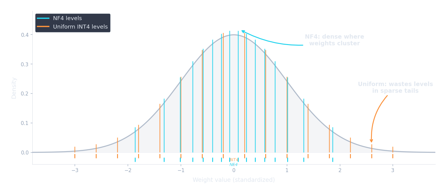
The code below computes and compares NF4 levels with uniform INT4 levels. Observa cómo NF4 packs levels tightly near zero (where the normal distribution is densest) and spreads them out in the tails (where few weights live).
import json, js, math

def norm_ppf(p):
    """Approximate inverse CDF of standard normal (Abramowitz & Stegun)."""
    if p <= 0: return -4.0
    if p >= 1: return 4.0
    if p > 0.5:
        return -norm_ppf(1.0 - p)
    t = math.sqrt(-2.0 * math.log(p))
    c0, c1, c2 = 2.515517, 0.802853, 0.010328
    d1, d2, d3 = 1.432788, 0.189269, 0.001308
    return -(t - (c0 + c1*t + c2*t*t) / (1 + d1*t + d2*t*t + d3*t*t*t))

bits = 4
n_levels = 2 ** bits  # 16

# NF4 levels: quantiles of N(0,1)
nf4_levels = []
for i in range(n_levels):
    p = (2 * i + 1) / (2 * n_levels)
    nf4_levels.append(norm_ppf(p))

# Uniform INT4 levels: evenly spaced over the same range
lo, hi = nf4_levels[0], nf4_levels[-1]
uniform_levels = [lo + i * (hi - lo) / (n_levels - 1) for i in range(n_levels)]

rows = []
for i in range(n_levels):
    p = (2 * i + 1) / (2 * n_levels)
    gap_nf4 = f"{nf4_levels[i] - nf4_levels[i-1]:.3f}" if i > 0 else "---"
    gap_uni = f"{uniform_levels[i] - uniform_levels[i-1]:.3f}" if i > 0 else "---"
    rows.append([
        str(i),
        f"{p:.5f}",
        f"{nf4_levels[i]:+.3f}",
        gap_nf4,
        f"{uniform_levels[i]:+.3f}",
        gap_uni,
    ])

js.window.py_table_data = json.dumps({
    "headers": ["Level i", "Prob p", "NF4 value", "NF4 gap", "Uniform value", "Uniform gap"],
    "rows": rows
})

print("NF4 levels cluster near zero (small gaps at center, large at tails)")
print("Uniform levels are equally spaced everywhere (gap always ~0.249)")
print(f"\nNF4 gap at center (i=7->8): {nf4_levels[8]-nf4_levels[7]:.3f}")
print(f"NF4 gap at tail  (i=0->1):  {nf4_levels[1]-nf4_levels[0]:.3f}")
print(f"Uniform gap everywhere: {uniform_levels[1]-uniform_levels[0]:.3f}")En la práctica, QLoRA normalizes each block of 64 weights by their absolute maximum before quantizing, so the actual NF4 levels are rescaled per block. But the core principle remains the same: match the cuantización grid to the data distribution, and you get dramáticamente less error with the same number of bits.
Doble Cuantización
NF4 reduces each weight from 16 bits to 4 bits — an impressive 4x compression. But there's a hidden cost: the scale factors . How much memory do they consume, and can we compress them too?
When we quantize a tensor, we don't apply a single global scale to the entire matriz de pesos. Instead, we divide the weights into small groups (typically 64 weights per group) and compute a separate FP32 scale factor $s$ for each group. This per-group scaling is essential because different parts of a matriz de pesos can have very different ranges — one group might span $[-0.2, +0.2]$ while another spans $[-1.5, +1.5]$. A single global scale would be too coarse for the first group and too fine for the second.
But the scale factors themselves consume memory. For each group of 64 weights, we store one FP32 scale factor (4 bytes = 32 bits). Let's calculate the overhead:
- 64 weights at 4 bits each: $64 \times 4 = 256$ bits $= 32$ bytes
- 1 FP32 scale factor: $32$ bits $= 4$ bytes
- Overhead: $4 / 32 = 12.5\%$, or equivalently $32 / 64 = 0.5$ extra bits per weight
So our effective storage is not 4.0 bits per weight but 4.5 bits. For a 70B model, that extra 0.5 bits adds up to $70 \times 10^9 \times 0.5 / 8 \approx 4.4$ GB — not trivial. QLoRA's double cuantización addresses this by quantizing the scale factors themselves.
Aquí está how it works. Instead of storing each scale factor as a 32-bit float, we collect scale factors into groups of 256 and quantize them to FP8 (8-bit floats) . Each group of 256 cuantizado scale factors shares a single FP32 second-level scale. The memory accounting per weight now becomes:
Let's evaluate each term. The first term is simply the 4 bits for the cuantizado weight itself. The second term divides the 8-bit cuantizado scale factor across the 64 weights in its group: $8/64 = 0.125$ bits per weight. The third term divides the 32-bit second-level scale across the $64 \times 256 = 16{,}384$ weights it ultimately covers: $32 / 16{,}384 \approx 0.00195$ bits per weight. Adding them up:
Converting to bytes: $4.127 / 8 \approx 0.516$ bytes per parameter. Compara esto with FP16 at 2.0 bytes per parameter — QLoRA achieves roughly a $2.0 / 0.516 \approx 3.88\times$ compression ratio. Without double cuantización, the overhead would be $4.5 / 8 = 0.5625$ bytes, so double cuantización saves about 8% of the total weight memory. That may sound small in percentage terms, but for a 70B model it means saving $70 \times 10^9 \times (0.5625 - 0.516) \approx 3.3$ GB — enough to fit a larger tamaño de batch or a longer sequence.
Optimizadores Paginados
Even with the base model compressed to 4 bits, can memory spikes during training still cause falta de memoria (OOM) crashes? Yes — and QLoRA includes a mechanism to handle them: paged optimizers .
During training, uso de memoria is not constant. It fluctuates depending on the tamaño de batch, the longitud de secuencia of the current batch, and whether techniques like gradient checkpointing are active (which trade compute for memory by recomputing activaciones during the paso backward instead of storing them). A batch of short sequences might use 30 GB of memoria de GPU, but a batch of long sequences might spike to 45 GB. If your GPU has 48 GB, that spike crashes the ejecución de entrenamiento — even though the average usage was well within budget.
Paged optimizers solve this by leveraging NVIDIA's unified memory feature, which allows memory to be automatically paged between GPU VRAM and CPU RAM — much like how an operating system uses swap space on disk when physical RAM runs out. Aquí está the analogy: your laptop has 16 GB of RAM but can run programs that collectively need 32 GB, because the OS silently swaps inactive pages to disk and brings them back when needed. Paged optimizers do the same thing between GPU and CPU memory.
When memoria de GPU pressure rises (say, during a paso forward on a long sequence), the estados del optimizador for LoRA parameters — which are needed only during the optimizer step, not during forward or paso backwardes — can be automatically paged out to CPU RAM. When the optimizer step runs, they page back in. This prevents OOM crashes at the cost of occasional latency from the CPU-GPU data transfer. En la práctica, the paging happens over PCIe and adds a few hundred milliseconds per paso de entrenamiento when triggered — noticeable, but far better than a crash.
Juntando Todo: Presupuesto de Memoria de QLoRA
Now that we understand all three components — NF4 cuantización, double cuantización, and paged optimizers — how much memory does QLoRA actually need? Recorramos a complete presupuesto de memoria for fine-tuning LLaMA-70B to see whether the promise of "70B on a single GPU" holds up.
The memory during training breaks down into four main categories:
1. Base model weights in NF4. With double cuantización, each parameter costs about 0.52 bytes. For 70 billion parameters: $70 \times 10^9 \times 0.52 \approx 36.4$ GB. Compara esto with FP16: $70 \times 10^9 \times 2 = 140$ GB. We've cut the base model from 140 GB to 36 GB.
2. LoRA adapters in FP16. With rank $r = 16$ applied to all linear layers in LLaMA-70B (which has 80 bloque transformers, each with 7 linear projections), the LoRA parameters total aproximadamente 160 million. At 2 bytes each in FP16: $160 \times 10^6 \times 2 \approx 0.32$ GB. Negligible.
3. Optimizer states for LoRA parameters. AdamW maintains two state vectors (first moment $m$ and second moment $v$) plus the gradient for each parámetro entrenable. That's roughly 12 bytes per parámetro entrenable (4 bytes each for gradient, $m$, and $v$ in FP32). For 160M LoRA parameters: $160 \times 10^6 \times 12 \approx 1.9$ GB. Aquí es donde LoRA's parameter efficiency pays off most — full fine-tuning of 70B would need $70 \times 10^9 \times 12 \approx 840$ GB just for estados del optimizador.
4. Activations and gradients. This depends heavily on tamaño de batch and longitud de secuencia. With gradient checkpointing, a tamaño de batch of 1, and a longitud de secuencia of 512 tokens, activaciones for a 70B model typically consume 5–10 GB. Increasing tamaño de batch or longitud de secuencia raises this proportionally.
Sumando todo: $36.4 + 0.32 + 1.9 + 7.5 \approx 46$ GB. That fits on a single 48 GB A6000 with a bit of headroom, or comfortably on an 80 GB A100. Compare with full fine-tuning of the same 70B model: $140$ (weights in FP16) $+ 840$ (estados del optimizador) $+ 280$ (gradients + master weights in FP32) $\approx 1{,}120$ GB — requiring a cluster of 16+ GPUs with paralelismo de modelo.
The table below compares memory requirements across model sizes and fine-tuning strategies:
import json, js

models = [
    ("LLaMA-7B",  7e9,  32, 7),
    ("LLaMA-13B", 13e9, 40, 7),
    ("LLaMA-70B", 70e9, 80, 7),
]

rows = []
for name, n_params, n_layers, n_linear in models:
    # Full fine-tuning (FP16 weights + FP32 optimizer states + gradients)
    full_ft_gb = n_params * 16 / 1e9  # ~16 bytes/param total

    # LoRA FP16 (base in FP16, LoRA adapters only)
    lora_params = n_layers * n_linear * 2 * 16 * 4096  # rough: r=16, d=4096 per proj
    if n_params > 30e9:
        lora_params = n_layers * n_linear * 2 * 16 * 8192  # 70B has d=8192
    lora_base_gb = n_params * 2 / 1e9         # base weights FP16
    lora_opt_gb = lora_params * 12 / 1e9       # optimizer for LoRA only
    lora_adapter_gb = lora_params * 2 / 1e9    # adapters in FP16
    lora_total_gb = lora_base_gb + lora_opt_gb + lora_adapter_gb + 5  # +5 for activations

    # QLoRA NF4 (base in NF4, LoRA adapters in FP16)
    qlora_base_gb = n_params * 0.52 / 1e9      # NF4 + double quant
    qlora_total_gb = qlora_base_gb + lora_opt_gb + lora_adapter_gb + 5  # +5 for activations

    rows.append([
        name,
        f"{n_params/1e9:.0f}B",
        f"{full_ft_gb:.0f} GB",
        f"{lora_total_gb:.1f} GB",
        f"{qlora_total_gb:.1f} GB",
    ])

js.window.py_table_data = json.dumps({
    "headers": ["Model", "Params", "Full FT (FP16+Adam)", "LoRA FP16", "QLoRA NF4"],
    "rows": rows
})

print("Full FT = 16 bytes/param (weights + grads + optimizer)")
print("LoRA FP16 = base in FP16 (2 B/param) + optimizer for adapters only")
print("QLoRA NF4 = base in NF4 (~0.52 B/param) + optimizer for adapters only")
print("All estimates include ~5 GB for activations (batch_size=1, seq_len=512)")
La diferencia es dramática. A 70B model goes from over 1 TB for full fine-tuning to under 50 GB with QLoRA — a reduction of more than 20x. And crucially, Dettmers et al. showed that this compression does not sacrifice quality . Their Guanaco-65B model, trained with QLoRA on just 24 hours of a single 48 GB GPU, achieved 99.3% of the performance of ChatGPT on the Vicuna benchmark. The quality gap between QLoRA and full 16-bit fine-tuning was statistically negligible across their evaluation suite.
QLoRA en la Práctica
How do we actually set up QLoRA in code? The standard toolchain combines three HuggingFace libraries:
bitsandbytes
(for cuantizado model loading),
peft
(for LoRA adapters), and
trl
(for supervised fine-tuning training). The configuration is straightforward — every concept we've discussed in this article maps directly to a parameter.
import torch
from transformers import AutoModelForCausalLM, AutoTokenizer, BitsAndBytesConfig
from peft import LoraConfig, get_peft_model, prepare_model_for_kbit_training
from trl import SFTTrainer, SFTConfig

# 1. Configure 4-bit quantization for the base model
bnb_config = BitsAndBytesConfig(
    load_in_4bit=True,                  # Load weights in 4-bit
    bnb_4bit_quant_type="nf4",          # Use NormalFloat4 (not uniform INT4)
    bnb_4bit_use_double_quant=True,     # Double quantization for scale factors
    bnb_4bit_compute_dtype=torch.bfloat16,  # Compute in BF16 during forward pass
)

# 2. Load the base model in quantized format
model = AutoModelForCausalLM.from_pretrained(
    "meta-llama/Llama-2-70b-hf",
    quantization_config=bnb_config,
    device_map="auto",                  # Automatically place layers on GPU
)
tokenizer = AutoTokenizer.from_pretrained("meta-llama/Llama-2-70b-hf")

# 3. Prepare model for k-bit training (freeze base, cast norms to FP32)
model = prepare_model_for_kbit_training(model)

# 4. Configure LoRA adapters (these train in FP16/BF16)
lora_config = LoraConfig(
    r=16,
    lora_alpha=32,
    target_modules="all-linear",        # Apply LoRA to every linear layer
    lora_dropout=0.05,
    bias="none",
    task_type="CAUSAL_LM",
)

# 5. Wrap model with LoRA
model = get_peft_model(model, lora_config)
model.print_trainable_parameters()
# => trainable params: ~160M || all params: ~70B || trainable%: ~0.23%

# 6. Train with SFTTrainer
training_args = SFTConfig(
    output_dir="./qlora-output",
    num_train_epochs=1,
    per_device_train_batch_size=1,
    gradient_accumulation_steps=16,     # Effective batch size = 16
    learning_rate=2e-4,
    bf16=True,                          # Mixed-precision training
    gradient_checkpointing=True,        # Trade compute for memory on activations
    optim="paged_adamw_8bit",           # Paged optimizer for memory spikes
    logging_steps=10,
    save_strategy="steps",
    save_steps=100,
    max_seq_length=512,
)

trainer = SFTTrainer(
    model=model,
    args=training_args,
    train_dataset=dataset,
    processing_class=tokenizer,
)

trainer.train()

# Save only the LoRA adapter (~300 MB, not the 35 GB quantized base)
model.save_pretrained("./qlora-adapter")
Recorramos the key configuration choices:
- bnb_4bit_quant_type="nf4" : selects NormalFloat4 cuantización instead of the default uniform INT4. As we discussed, NF4 places cuantización levels at the quantiles of a normal distribution, matching the empirical distribution of LLM weights.
- bnb_4bit_use_double_quant=True : enables double cuantización, reducing the per-weight overhead of scale factors from 0.5 bits to about 0.127 bits.
- bnb_4bit_compute_dtype=torch.bfloat16 : this is critical. Although the base weights are stored in NF4, all matrix multiplications happen in BF16. During the paso forward, each block of 64 weights is decuantizado to BF16 on the fly before the computation. This ensures numerical stability — you'd get poor gradients if you tried to compute in 4-bit precision.
- optim="paged_adamw_8bit" : uses the paged 8-bit AdamW optimizer. The "8bit" part means estados del optimizador ($m$ and $v$) are stored in 8-bit format instead of FP32, further reducing memory. The "paged" part enables CPU-memoria de GPU paging for handling spikes.
- gradient_checkpointing=True : instead of storing all intermediate activaciones during the paso forward (which would require tens of GB), gradient checkpointing recomputes them during the paso backward. This roughly halves memoria de activaciones at the cost of about 30% more compute time.
QLoRA, together with LoRA, forms the backbone of modern de eficiencia de parámetros fine-tuning. By quantizing the modelo base congelado and training only low-rank adapters in precisión completa, QLoRA makes it possible to hacer fine-tuning the largest open-source LLMs on a single GPU — democratizing model adaptation in a way that was unimaginable when these models were released. LoRA and QLoRA are the most popular PEFT methods in practice, but the landscape of efficient adaptation continues to evolve with methods like DoRA, AdaLoRA, and others.
Pruébalo Tú Mismo
Want to see QLoRA in action? This notebook loads a model in NF4, applies LoRA, hacer fine-tunings on an instruction dataset, and merges the result — all on a free T4 GPU.
Quiz
Test your understanding of QLoRA's cuantización techniques and memory optimizations.
Why does NF4 cuantización place cuantización levels at the quantiles of a normal distribution rather than spacing them uniformly?
What does double cuantización compress, and why does it help?
During QLoRA training, in what precision do the actual matrix multiplications happen?
A 70B-parameter model in QLoRA (NF4 + double cuantización) uses aproximadamente how much memory for the base weights, and how does this compare to FP16?