The PEFT Landscape

Beyond LoRA: Why One Method Isn't Enough

In article 3, we covered LoRA in detail: freeze the base model, inject low-rank matrices, and train only those. It's clean, efficient, and by far the most popular parameter-efficient fine-tuning (PEFT) method. So why bother learning about anything else?

Because different methods make different trade-offs. LoRA is excellent in most settings, but it isn't universally optimal. Some methods use fewer parameters. Others avoid inference overhead entirely. Some shine when you have very few training examples. And some capture aspects of the weight update that LoRA systematically misses. Knowing the full landscape lets you pick the right tool when LoRA's default trade-off doesn't match your constraints.

Every PEFT method answers the same fundamental question differently: "Which small subset of the model should we modify, and how?" The methods fall into three families:

• Additive methods: inject entirely new parameters into the architecture. The base model is frozen and the new parameters provide extra computation that steers the model's behaviour. Adapters, prefix tuning, and prompt tuning all belong here.
• Reparameterization methods: decompose or restructure the weight update rather than adding new modules. LoRA and DoRA are the main examples: they don't add layers, they express the weight change in a more compact form.
• Selective methods: choose which existing parameters to update and freeze the rest. This includes strategies like freezing all layers except the last few, or training only bias terms. IA$^3$ sits at the boundary: it multiplies activations by learned scalars, which can be viewed as selectively rescaling existing features.

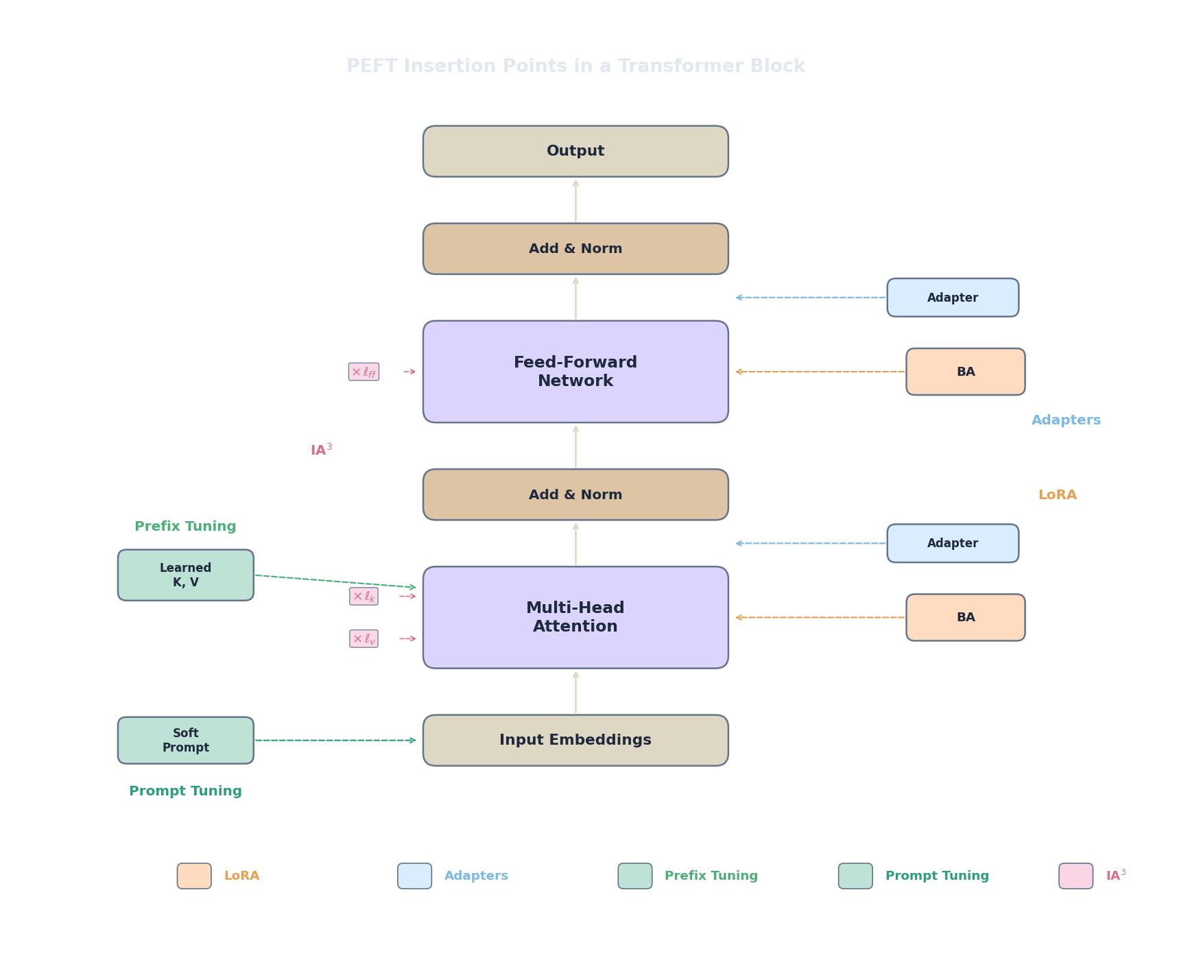
We'll walk through the most important methods in each family, starting with the one that predates LoRA: adapters.

Adapters: Bottleneck Layers Inside the Transformer

What if, instead of decomposing the weight update, we inserted small trainable modules directly into the transformer architecture? That's the adapter approach, introduced by (Houlsby et al., 2019) . The core idea is disarmingly simple: add a tiny bottleneck network after the attention sublayer and after the feed-forward sublayer in every transformer block, then freeze everything else and train only these inserted modules.

Each adapter module has the same architecture: project down to a small dimension, apply a nonlinearity, project back up, and add a residual connection. The forward pass through one adapter looks like this:

Let's unpack each piece.

$h \in \mathbb{R}^d$ is the hidden state — the output of the preceding sublayer (either attention or FFN). The adapter takes this as input and produces a modified version.

$W_{\text{down}} \in \mathbb{R}^{d \times r}$ is the down-projection matrix. It compresses the $d$-dimensional hidden state to a much smaller $r$-dimensional representation, where $r \ll d$. This is the bottleneck: all adaptation information must pass through these $r$ channels. The vector $b_{\text{down}} \in \mathbb{R}^r$ is the corresponding bias.

$f$ is a nonlinear activation function (typically ReLU or GELU). This is a crucial difference from LoRA, which has no nonlinearity. The activation allows the adapter to learn nonlinear transformations of the hidden state, making each adapter module more expressive per parameter than a simple linear projection.

$W_{\text{up}} \in \mathbb{R}^{r \times d}$ is the up-projection matrix. It maps the $r$-dimensional bottleneck representation back to $d$ dimensions so it can be added to the original hidden state. The vector $b_{\text{up}} \in \mathbb{R}^d$ is the corresponding bias.

The $+ \, h$ at the beginning is the residual connection . If the adapter weights are initialized near zero, then the adapter output is approximately zero and the whole expression reduces to $h + 0 = h$ — the adapter starts as an identity function and gradually learns to nudge the hidden state during training. This is the same principle as LoRA's zero-initialization of $B$: begin where pre-training left off.

Now let's look at the boundaries. When $r = d$ (no bottleneck), the adapter has full capacity to represent any transformation of $h$, but we've gained nothing in parameter efficiency. When $r = 1$, the entire adaptation at that position is controlled by a single hidden unit — extremely compressed but very limited. In practice, $r$ is typically set between 8 and 64, mirroring LoRA's rank choices.

Each adapter is placed at two positions per transformer block: one after the multi-head attention sublayer and one after the feed-forward sublayer. For a model with $L$ transformer layers, the total trainable parameter count is:

The outer factor of 2 accounts for the two adapter positions per layer (post-attention and post-FFN). The inner factor of 2 accounts for the two matrices ($W_{\text{down}}$ and $W_{\text{up}}$) in each adapter module. The $d \times r$ counts the elements in one matrix (biases add the $+ r$ term, since each bias has $r$ or $d$ elements, but the dominant cost is the matrices). For a model with $d = 4096$, $r = 64$, and $L = 32$ layers, this comes to $2 \times 32 \times 2 \times (4096 \times 64 + 64) \approx 33.6\text{M}$ trainable parameters — comparable to LoRA.

Here's a minimal adapter module implemented in PyTorch:

import torch
import torch.nn as nn

class AdapterModule(nn.Module):
    """A bottleneck adapter inserted after a transformer sublayer."""
    def __init__(self, d_model: int, bottleneck: int = 64):
        super().__init__()
        self.down = nn.Linear(d_model, bottleneck)   # W_down: d -> r
        self.activation = nn.GELU()
        self.up = nn.Linear(bottleneck, d_model)      # W_up:  r -> d

        # Initialize near zero so the adapter starts as identity
        nn.init.zeros_(self.up.weight)
        nn.init.zeros_(self.up.bias)

    def forward(self, h):
        # Residual connection: h + adapter(h)
        return h + self.up(self.activation(self.down(h)))

# Example: adapter for a model with d_model=4096, bottleneck=64
adapter = AdapterModule(d_model=4096, bottleneck=64)

params = sum(p.numel() for p in adapter.parameters())
print(f"Adapter parameters: {params:,}")
# W_down: 4096*64 + 64 = 262,208
# W_up:   64*4096 + 4096 = 266,240
# Total:  528,448 per adapter module
print(f"Per transformer block (2 adapters): {params * 2:,}")
print(f"For 32-layer model: {params * 2 * 32:,}")

Notice the zero initialization of the up-projection: this ensures the adapter output starts at zero, preserving the base model's behaviour at the beginning of training. The down-projection uses default initialization because the zero output from the up-projection already guarantees identity behaviour.

Prefix Tuning: Learned Context Vectors

Adapters modify the model by inserting new computation. But what if we could steer the model without changing its architecture at all — by changing what it sees instead of what it does ?

That's the idea behind prefix tuning (Li & Liang, 2021) . Instead of modifying any weights, we prepend a set of learnable virtual tokens to the key and value matrices in every attention layer. These virtual tokens have no corresponding input text — they are free parameters that the model learns to attend to. The entire base model stays frozen; only the prefix vectors are trained.

Concretely, for each attention layer $l$, we prepend a learned prefix matrix $P_K^{(l)} \in \mathbb{R}^{p \times d}$ to the key matrix and $P_V^{(l)} \in \mathbb{R}^{p \times d}$ to the value matrix, where $p$ is the prefix length (typically 10 to 100 virtual tokens) and $d$ is the model's hidden dimension. The attention computation becomes:

Here $[P_K; K]$ means we concatenate the prefix keys with the actual keys along the sequence dimension, and similarly for the values. Every query token can now attend to both the real input tokens and the $p$ virtual prefix tokens. Since the prefix has no corresponding input, the model has full freedom to learn whatever key-value vectors are most useful for steering the output toward the target task.

The total number of trainable parameters is:

The factor of 2 accounts for both the key prefix $P_K$ and the value prefix $P_V$ at each layer. $L$ is the number of transformer layers, $p$ is the prefix length, and $d$ is the hidden dimension. For a model with $L = 32$, $d = 4096$, and $p = 20$, this gives $2 \times 32 \times 20 \times 4096 = 5{,}242{,}880$ parameters — about 5.2M, which is quite small.

Let's check the boundaries. When $p = 0$: no prefix tokens exist, the model sees only the real input, and behaviour is identical to the frozen base model. When $p$ is very large: the model has many virtual tokens to attend to, giving it more capacity to steer behaviour, but the real tokens now compete with $p$ prefix tokens for attention weight, diluting their influence. And critically, each prefix token occupies one position in the sequence, so $p$ prefix tokens reduce the effective context length by $p$. With a 2048-token context window and $p = 100$, you only have 1948 tokens left for actual input.

In practice, Li & Liang found that directly optimizing the prefix vectors can be unstable — the loss landscape is sharp and training is sensitive to initialization. Their solution is to reparameterize the prefix through a small MLP during training: instead of directly learning $P_K^{(l)}$ and $P_V^{(l)}$, they learn a smaller set of vectors and map them through a two-layer feed-forward network to produce the actual prefix. After training completes, the MLP is discarded and only the resulting prefix vectors are kept for inference.

Prompt Tuning: The Simplest PEFT Method

If prefix tuning adds learned vectors to every layer, could we simplify even further and add them to just the input ? That's exactly what prompt tuning does (Lester et al., 2021) . Instead of injecting learnable vectors at every layer, we prepend $p$ learnable embedding vectors to the input sequence only. The rest of the model is completely frozen.

The input to the model becomes:

Here $e_i \in \mathbb{R}^d$ are the learned soft prompt embeddings ($p$ of them), and $x_1, \ldots, x_n$ are the regular input token embeddings. The word "soft" distinguishes these continuous, learned vectors from the discrete text tokens of a hand-written prompt (which would be "hard" prompt tuning). The soft prompt vectors live in the same embedding space as real tokens but aren't constrained to correspond to any word in the vocabulary.

The parameter count is remarkably small:

No per-layer additions, no matrices — just $p$ vectors of dimension $d$. For $p = 20$ and $d = 4096$, that's $20 \times 4096 = 81{,}920$ parameters. Compare that to LoRA's millions or even prefix tuning's 5M+ parameters. Prompt tuning is by far the most parameter-efficient method on this list.

But there's a catch, and it's a big one. At small model scales (under ~1B parameters), prompt tuning performs significantly worse than LoRA, adapters, or even full fine-tuning. With only a few soft tokens prepended to the input, the model simply doesn't have enough signal to adapt its deep internal representations. The soft prompt influences the first layer directly, but its effect on deeper layers is indirect (filtered through the frozen attention and FFN computations), and that indirection loses information.

The key finding from Lester et al. is that this gap closes as models get larger. At 10B+ parameters, prompt tuning approaches the performance of full fine-tuning. Why? Larger models have richer internal representations and more powerful attention mechanisms. A few well-placed soft tokens at the input are enough to activate the right "circuits" deep inside the model, because the model is already capable of complex conditional behaviour — it just needs a small nudge at the input to trigger it.

One practical advantage of prompt tuning is multi-task serving. Since the model itself is completely untouched, you can swap tasks by simply swapping the soft prompt prefix — even within the same batch. Different requests can use different soft prompts while sharing the exact same model weights. This is even cheaper than LoRA adapter swapping, because there are no per-layer components to load.

IA3: Rescaling Instead of Adding

All the methods we've seen so far add something to the model: extra matrices (LoRA, adapters), extra tokens (prefix and prompt tuning). IA3 (Infused Adapter by Inhibiting and Amplifying Inner Activations) (Liu et al., 2022) takes a fundamentally different approach: instead of adding new computation, it multiplies existing activations by learned scaling vectors.

Specifically, IA3 introduces three learned vectors per transformer layer. For the key projection, value projection, and feed-forward output:

Let's break down what each piece does.

$l_k, l_v \in \mathbb{R}^d$ are learned vectors with one scalar per feature dimension, applied to the key and value projections respectively. The symbol $\odot$ denotes element-wise (Hadamard) multiplication : each scalar in the learned vector multiplies the corresponding dimension of the activation. Think of it as a per-feature volume knob.

$l_{\text{ff}} \in \mathbb{R}^{d_{\text{ff}}}$ is the learned scaling vector for the feed-forward sublayer output, where $d_{\text{ff}}$ is the FFN's intermediate dimension. The function $f(x)$ represents the feed-forward sublayer's output before the final projection.

Now the boundary analysis reveals the elegance of this design:

• When $l_i = 1$ for all $i$: $l \odot a = a$, so the scaling is an identity operation. The model behaves exactly like the frozen base model. This is where IA3 starts (all vectors initialized to ones).
• When $l_i = 0$: that feature dimension is completely suppressed — zeroed out. The model loses all information carried in that dimension. This is "inhibiting" in the IA3 name.
• When $l_i > 1$: that feature dimension is amplified beyond its original magnitude. The model pays more attention to that dimension than it did during pre-training. This is "amplifying" in the IA3 name.
• When $0 < l_i < 1$: partial suppression. The feature is dampened but not eliminated.

The total parameter count is minimal:

For each of the $L$ transformer layers, we store two vectors of dimension $d$ (for keys and values) and one vector of dimension $d_{\text{ff}}$ (for the FFN output). For a model with $L = 32$, $d = 4096$, and $d_{\text{ff}} = 11008$, this gives $32 \times (2 \times 4096 + 11008) = 614{,}400$ parameters — about 0.6M. That's roughly 100 times fewer parameters than a typical LoRA configuration.

So when does IA3 shine? In few-shot fine-tuning scenarios where you have very little training data (tens to low hundreds of examples). Liu et al. showed that IA3 combined with few-shot learning outperformed in-context learning (putting examples directly in the prompt) on a range of tasks while using no context-window space at inference time. When data is scarce, the ultra-low parameter count of IA3 acts as a strong regularizer that prevents overfitting.

Like LoRA (and unlike adapters), IA3's scaling can be absorbed into the base weights at inference time. For the key projection, for example, $l_k \odot W_K x = (\text{diag}(l_k) \cdot W_K) x$. We can precompute $W_K' = \text{diag}(l_k) \cdot W_K$ and replace the original weight, so there is no inference overhead .

DoRA: Decomposing Weight Updates Directionally

If we zoom in on what happens during full fine-tuning, we can observe that the weight vectors change in two distinct ways: they change in magnitude (how large the weights are) and in direction (where they point in parameter space). (Liu et al., 2024) analysed this pattern carefully and found something striking: LoRA primarily changes direction but underperforms at adapting magnitude. Full fine-tuning, in contrast, adjusts both freely. This mismatch suggests a simple improvement: what if we decompose the weight update into magnitude and direction explicitly?

That's DoRA (Weight-Decomposed Low-Rank Adaptation) . It rewrites the weight matrix as:

Let's unpack every symbol.

$m \in \mathbb{R}^d$ is a learnable magnitude vector with one scalar per output neuron. It controls how "strong" each output dimension is, independently of where the weight vector points. Think of it as a per-neuron volume knob (similar in spirit to IA3, but applied to the weight matrix rather than to activations).

$V \in \mathbb{R}^{d \times k}$ is the directional matrix . In DoRA, this is not learned from scratch — it starts from the pre-trained weight $W_0$ and receives a LoRA-style low-rank update:

where $B \in \mathbb{R}^{d \times r}$ and $A \in \mathbb{R}^{r \times k}$ are the same low-rank matrices from LoRA. So the directional component is updated via LoRA, while the magnitude gets its own dedicated learnable vector.

$\|V\|_c$ denotes the column-wise norm : for each column of $V$ (corresponding to one output neuron), we compute its L2 norm. Dividing by this norm gives a unit-length direction vector. The magnitude $m$ then rescales each output neuron to the desired length. This decomposition ensures that $m$ controls only magnitude and $V / \|V\|_c$ controls only direction — the two aspects are cleanly separated.

Why does this help? Consider what happens during LoRA fine-tuning. The update $\Delta W = BA$ is a rank-$r$ matrix that shifts the weight in a low-dimensional subspace. Because both magnitude and direction are entangled in this single matrix product, LoRA can't independently scale one neuron louder while pointing another in a completely different direction. DoRA decouples these two controls. The LoRA matrices $B$ and $A$ handle the directional update (where should each neuron point?), while $m$ handles the magnitude update (how strong should each neuron be?). Since Liu et al. observed that full fine-tuning adjusts both freely, giving the adapter the same two degrees of freedom more closely mimics full fine-tuning's update pattern.

At the boundaries: if $m$ equals the column norms of $W_0$ and $BA = 0$, DoRA reduces to the original pre-trained weight (identity initialization). If $m \to 0$ for some output neuron, that neuron is silenced entirely. If the LoRA component $BA$ is large relative to $W_0$, the direction of the weight vectors shifts dramatically — same as standard LoRA, but now with independent magnitude control on top.

The parameter overhead compared to LoRA is minimal: just the $d$-dimensional magnitude vector $m$ per adapted layer. For a model with $d = 4096$ and 32 layers, that's only $32 \times 4096 = 131{,}072$ extra parameters — negligible compared to LoRA's millions.

Here's how to use DoRA with HuggingFace PEFT — notice how little changes from a standard LoRA configuration:

from peft import LoraConfig, get_peft_model
from transformers import AutoModelForCausalLM

model = AutoModelForCausalLM.from_pretrained("meta-llama/Llama-2-7b-hf")

# Standard LoRA config — with one extra flag for DoRA
config = LoraConfig(
    r=16,
    lora_alpha=32,
    target_modules=["q_proj", "k_proj", "v_proj", "o_proj",
                     "gate_proj", "up_proj", "down_proj"],
    use_dora=True,   # <-- This is the only change from standard LoRA
    task_type="CAUSAL_LM",
)

peft_model = get_peft_model(model, config)
peft_model.print_trainable_parameters()
# Output: trainable params: ~40M | all params: ~6.7B | trainable%: ~0.60%
# (slightly more than LoRA due to the magnitude vectors)

The training loop, optimizer, and all other settings remain identical to LoRA. DoRA is a strict upgrade in most scenarios — slightly more parameters for measurably better performance.

Choosing the Right Method

With five PEFT methods on the table (adapters, prefix tuning, prompt tuning, IA3, and the LoRA/DoRA family), how do you choose? The decision comes down to four factors: parameter count, inference overhead, the amount of training data, and the quality ceiling you need. The following comparison summarizes the trade-offs:

import json, js

# Comparison table: PEFT methods at a glance
# Assumes a 7B-parameter model with d=4096, L=32, d_ff=11008

rows = [
    ["LoRA (r=16)",        "~40M (0.6%)",    "None (mergeable)",     "Fast",     "Default choice; best balance of quality and efficiency"],
    ["DoRA (r=16)",        "~40M (0.6%)",    "None (mergeable)",     "Fast",     "Maximum quality; drop-in LoRA upgrade"],
    ["Adapters (r=64)",    "~34M (0.5%)",    "Added latency",        "Fast",     "Legacy systems needing separate inference modules"],
    ["Prefix tuning (p=20)", "~5M (0.08%)",  "Reduced context",      "Fast",     "Generation tasks with limited parameters"],
    ["Prompt tuning (p=20)", "~82K (0.001%)", "Reduced context",     "Fast",     "10B+ models; ultra-cheap multi-task serving"],
    ["IA3",                "~0.6M (0.01%)",  "None (mergeable)",     "Fastest",  "Few-shot fine-tuning with very little data"],
]

js.window.py_table_data = json.dumps({
    "headers": ["Method", "Params (7B model)", "Inference Overhead", "Training Speed", "Best For"],
    "rows": rows
})

print("PEFT method comparison for a 7B-parameter model (d=4096, L=32)")
print("LoRA and DoRA can be merged into base weights => zero inference cost")
print("Adapters add sequential computation => measurable latency increase")
print("Prefix/prompt tuning consume sequence positions => less room for input")

A few rules of thumb that have emerged from the community:

• Default choice: LoRA. Best balance of quality, efficiency, and ecosystem support. The vast majority of PEFT practitioners start here, and for good reason — it works well across tasks, has extensive tooling, and adds zero inference cost after merging.
• Memory-constrained: QLoRA. Combine LoRA with 4-bit quantization (covered in article 4) when GPU memory is tight. You get LoRA's quality with a fraction of the memory footprint.
• Very few examples: IA3 or prompt tuning. When you have only tens of labelled examples, the ultra-low parameter count of these methods acts as a strong regularizer. IA3 in particular was designed for few-shot settings and consistently outperforms in-context learning there.
• Maximum quality: DoRA. When you want the best possible fine-tuned model and can afford marginally more complexity, DoRA's magnitude-direction decomposition consistently outperforms LoRA at the same rank.
• Legacy or modular systems: Adapters. If your deployment requires separate, hot-swappable inference modules and you cannot merge weights (e.g., regulatory constraints that require auditing the exact adapter), adapters keep the base model provably untouched.

Regardless of which PEFT method you choose, there's a factor that matters more than any of them: the quality of your training data. A perfect LoRA configuration trained on noisy, poorly formatted data will produce a worse model than a basic configuration trained on clean, well-curated examples. That's what the next article is about — how to prepare the data that actually drives fine-tuning quality.

Quiz

Test your understanding of the PEFT landscape and the trade-offs between methods.