Distributed Fine-tuning

When One GPU Isn't Enough

Back in article 2 we counted the bytes: a 7B model under full fine-tuning with AdamW needs roughly $16N = 112$ GB of GPU memory just for weights, gradients, and optimiser states — more than a single A100-80GB can hold. Scale to 70B parameters and the bill explodes to $16 \times 70\text{B} = 1.12$ TB. Even with the memory savings from QLoRA (article 4), a 70B model still demands about 35 GB for the 4-bit base weights alone, and the training state ( LoRA gradients, optimiser moments, activations) pushes the total higher. At some point, one GPU simply cannot hold everything.

The obvious answer is to use more GPUs. But plugging in a second card and hoping for the best doesn't work — the training loop still tries to load the full model onto a single device. Multiple GPUs are useless without a strategy for splitting the work . That strategy must decide two things: what data goes where, and what model state goes where. Every approach in this article is some combination of those two decisions.

At the highest level there are two fundamental strategies. The first is data parallelism : give every GPU a full copy of the model and split the training data across them, so each GPU processes different examples. The second is model parallelism : split the model itself across GPUs, so each device holds only a fraction of the parameters. In practice, the most powerful systems combine both ideas — and the particular flavour of combination you choose determines how much memory you save, how much communication overhead you pay, and how large a model you can fine-tune.

Data Parallelism (DDP)

How do we get $N$ GPUs to train a model faster without changing the model itself? The simplest answer is Distributed Data Parallel (DDP) (Li et al., 2020) . The idea is straightforward: every GPU holds a complete copy of the model. At each training step, the global mini-batch is split into $N$ equal chunks, one per GPU. Each GPU runs forward and backward passes on its own chunk independently, producing a set of local gradients. Then, before the optimiser updates the weights, the GPUs communicate to average their gradients so that every device applies the same update and stays in sync.

That gradient-averaging step is called an all-reduce operation. In a naive implementation, every GPU would send its full gradient tensor to every other GPU — an $O(N^2)$ communication nightmare. The standard solution is the ring all-reduce algorithm, which arranges GPUs in a logical ring and completes the operation in two phases: a reduce-scatter phase (where each GPU accumulates partial sums for different gradient chunks) followed by an all-gather phase (where each GPU broadcasts its final chunk to everyone else). The total data transferred per GPU is:

Let's unpack every piece of this. $N$ is the number of GPUs, and $M$ is the total size of the gradient tensor in bytes (for a model with $P$ parameters in FP16, $M = 2P$). The factor $\frac{2(N-1)}{N}$ comes from the two phases of ring all-reduce: the reduce-scatter phase transfers $\frac{N-1}{N} \times M$ bytes per GPU (each GPU sends $N-1$ chunks out of the $N$ total chunks of the gradient), and the all-gather phase transfers the same $\frac{N-1}{N} \times M$ bytes. Multiplying by 2 gives the total.

The boundary behaviour is revealing. With $N = 2$ GPUs: $\frac{2 \times 1}{2} \times M = M$ bytes per GPU — each GPU transfers exactly one copy of the full gradient. With $N = 8$: $\frac{2 \times 7}{8} \times M = 1.75M$ bytes per GPU. And as $N \to \infty$, the factor approaches $2M$. This means communication cost per GPU is bounded — it does not grow linearly with the number of GPUs. Adding more GPUs increases total parallelism without proportionally increasing each GPU's communication burden. That's what makes ring all-reduce so scalable.

With DDP, the effective batch size scales linearly with the number of GPUs:

If each GPU processes $b_{\text{per\_gpu}} = 4$ examples and you have $N_{\text{gpus}} = 8$ GPUs, the effective batch size is 32. This is identical to training on a single GPU with batch size 32 — the gradients are mathematically the same (up to floating-point rounding). The benefit is speed: 8 GPUs process 8 chunks simultaneously, so each step takes roughly the same wall-clock time as a single GPU processing one chunk.

Here is the problem with DDP: every GPU stores the full model plus all optimiser states . For a 7B model, that's 112 GB per GPU — weights, gradients, optimiser moments, the lot. If you have 8 A100-80GB GPUs, DDP replicates the optimiser state 8 times. Seven of those copies are pure waste: every GPU computes the same update and arrives at the same weights. We're paying 8 times the memory to get 8 times the throughput, when ideally we'd want the memory burden to decrease as we add GPUs. This redundancy is exactly what ZeRO eliminates.

DeepSpeed ZeRO: Eliminating Redundancy

If DDP wastes memory by replicating everything, the natural fix is to stop replicating. ZeRO (Zero Redundancy Optimizer) (Rajbhandari et al., 2020) does exactly that. Instead of giving every GPU a full copy of the optimizer states, gradients, and parameters, ZeRO shards (partitions) them across GPUs so that each device stores only $1/N$ of the state it would normally hold. When a GPU needs a piece of state it doesn't own — say, the parameters of a particular layer for the forward pass — it gathers them from the GPU that does own them, uses them, and discards them. The memory savings are enormous; the cost is communication.

ZeRO comes in three stages, each progressively more aggressive about what gets sharded. In all formulas below, $P$ is the number of model parameters, $N$ is the number of GPUs, and we use the standard mixed-precision AdamW memory breakdown from article 2: $2P$ bytes for FP16 model weights, $2P$ bytes for FP16 gradients, and $12P$ bytes for FP32 optimiser states (master weights + first moment + second moment).

ZeRO Stage 1 (ZeRO-1) shards only the optimiser states. Each GPU stores the full model weights ($2P$), the full gradients ($2P$), but only $1/N$ of the optimiser states ($12P/N$). Memory per GPU:

For 7B parameters on 8 GPUs: $4 \times 7\text{B} + \frac{12 \times 7\text{B}}{8} = 28 + 10.5 = 38.5$ GB per GPU. That fits on a single A100-80GB with room to spare for activations. Compare this to the 112 GB that standard DDP demands — ZeRO-1 cuts memory by nearly 3x on 8 GPUs, and all we gave up is the locality of optimiser states.

ZeRO Stage 2 (ZeRO-2) shards both the optimiser states and the gradients. Each GPU stores the full model weights ($2P$), but only $1/N$ of the gradients ($2P/N$) and $1/N$ of the optimiser states ($12P/N$). Memory per GPU:

For 7B on 8 GPUs: $2 \times 7\text{B} + \frac{14 \times 7\text{B}}{8} = 14 + 12.25 = 26.25$ GB per GPU. We've dropped another 12 GB compared to ZeRO-1. The gradient sharding works naturally with the reduce-scatter phase of all-reduce: instead of all-gathering the fully reduced gradients back to every GPU (as DDP does), each GPU keeps only the $1/N$ shard it's responsible for. There's no extra communication cost beyond what DDP already pays.

ZeRO Stage 3 (ZeRO-3) shards everything : parameters, gradients, and optimiser states. Each GPU stores only $1/N$ of the entire training state:

For 7B on 8 GPUs: $\frac{16 \times 7\text{B}}{8} = 14$ GB per GPU. That's a fraction of what DDP requires. But more impressively, this formula means a 70B model on 8 GPUs needs $\frac{16 \times 70\text{B}}{8} = 140$ GB total, or just 17.5 GB per GPU. A model that would need over a terabyte under DDP now fits comfortably on 8 A100-80GB cards.

The tradeoff is communication. Since no GPU holds the full parameter set, ZeRO-3 must gather parameters on the fly during both the forward and backward passes. Before computing a layer's output, the GPU broadcasts a request for that layer's parameters, uses them, and then discards them to free memory. This adds an all-gather operation per layer per pass, increasing communication volume by roughly 1.5x compared to standard DDP. Whether this overhead matters depends on the interconnect speed between your GPUs — on NVLink-connected A100s (600 GB/s bidirectional), it's barely noticeable; on PCIe-connected consumer cards, it can become a bottleneck.

Let's check the boundary cases. With $N = 1$ GPU, ZeRO-3 gives $16P/1 = 16P$ bytes — exactly the same as standard DDP. No sharding benefit with a single device, as expected. As $N$ grows, memory per GPU drops as $1/N$: double the GPUs, halve the per-device memory. This linear scaling is why ZeRO-3 is the go-to strategy for fine-tuning models that are too large for a single node.

The following calculator shows the memory per GPU for each ZeRO stage across a range of model sizes and GPU counts, so you can quickly see which stage fits your hardware.

import json, js

def mem_per_gpu(P_billions, N_gpus, stage):
    """Memory in GB per GPU for a given ZeRO stage.
    P_billions: parameter count in billions
    N_gpus: number of GPUs
    stage: 0 (DDP), 1, 2, or 3
    """
    P = P_billions  # keep in billions, result in GB
    if stage == 0:    # DDP: full replication
        return 2*P + 2*P + 12*P           # 16P
    elif stage == 1:  # shard optimizer only
        return 2*P + 2*P + 12*P / N_gpus  # 4P + 12P/N
    elif stage == 2:  # shard optimizer + gradients
        return 2*P + (2*P + 12*P) / N_gpus  # 2P + 14P/N
    elif stage == 3:  # shard everything
        return (2*P + 2*P + 12*P) / N_gpus  # 16P/N

rows = []
for model_name, P in [("7B", 7), ("70B", 70)]:
    for N in [4, 8]:
        for stage in [0, 1, 2, 3]:
            mem = mem_per_gpu(P, N, stage)
            fits = "Yes" if mem <= 80 else "No"
            rows.append([
                model_name,
                str(N),
                f"Stage {stage}" if stage > 0 else "DDP",
                f"{mem:.1f} GB",
                fits
            ])

js.window.py_table_data = json.dumps({
    "headers": ["Model", "GPUs", "Strategy", "Memory/GPU", "Fits A100-80GB?"],
    "rows": rows
})

print("Memory per GPU for weights + gradients + optimizer (no activations)")
print("Assumes mixed-precision AdamW (16P bytes total)")
print()
print("Key insight: ZeRO-3 with 8 GPUs brings 70B down to 17.5 GB/GPU")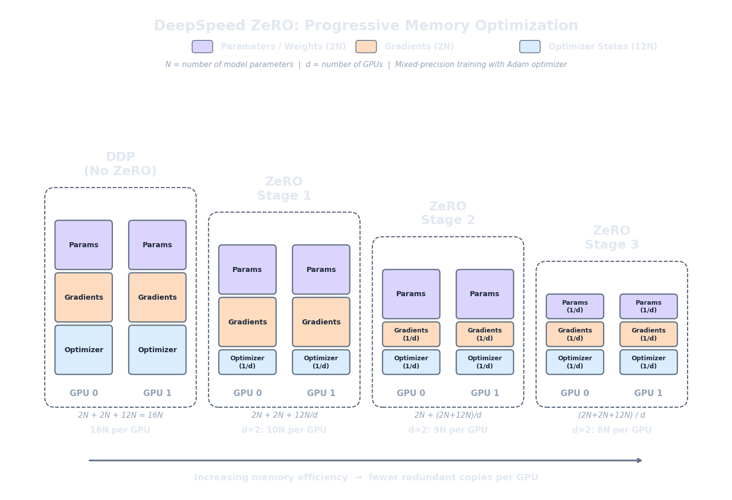

FSDP: PyTorch-Native Sharding

DeepSpeed ZeRO requires installing a separate library and writing JSON configuration files. For teams already deep in the PyTorch ecosystem, this friction led to a natural question: can we get the same memory savings natively? Fully Sharded Data Parallel (FSDP) (Zhao et al., 2023) is PyTorch's answer. It implements the same core idea as ZeRO-3 — shard parameters, gradients, and optimiser states across GPUs — but as a first-class PyTorch API, using the same torch.distributed primitives that DDP uses.

FSDP wraps each module (or group of modules) in a sharding unit. Before the forward pass of a sharding unit, FSDP runs an all-gather to reconstruct the full parameters from all GPUs. After the forward pass, the non-owned parameters are freed. During the backward pass, parameters are gathered again, gradients are computed, and then a reduce-scatter distributes gradient shards back to their owners. The memory profile is identical to ZeRO-3: at any given moment, only one layer's full parameters are materialised, and the rest exist as $1/N$ shards.

FSDP exposes three sharding strategies that map directly to the ZeRO stages:

• FULL_SHARD: equivalent to ZeRO-3. Shards parameters, gradients, and optimiser states. Maximum memory savings, highest communication.
• SHARD_GRAD_OP: equivalent to ZeRO-2. Shards gradients and optimiser states but keeps full parameters on each GPU. Less communication than FULL_SHARD since parameters don't need to be gathered for the forward pass.
• NO_SHARD: plain DDP. No sharding at all — every GPU holds everything. Useful as a baseline or when the model already fits in memory and you want maximum throughput.

In code, wrapping a model with FSDP requires minimal changes compared to DDP. The key difference is specifying the sharding strategy and the auto_wrap_policy , which tells FSDP how to group layers into sharding units. Typically you wrap at the transformer-block level (each block becomes one sharding unit), so parameters are gathered and freed one block at a time:

import torch
from torch.distributed.fsdp import (
    FullyShardedDataParallel as FSDP,
    ShardingStrategy,
)
from torch.distributed.fsdp.wrap import transformer_auto_wrap_policy
from transformers import AutoModelForCausalLM, LlamaDecoderLayer

# Load model on CPU first (FSDP will shard onto GPUs)
model = AutoModelForCausalLM.from_pretrained("meta-llama/Llama-2-7b-hf")

# Define wrapping policy: shard at each transformer block
wrap_policy = transformer_auto_wrap_policy(
    transformer_layer_cls={LlamaDecoderLayer}
)

# Wrap with FSDP (FULL_SHARD = ZeRO-3 equivalent)
model = FSDP(
    model,
    sharding_strategy=ShardingStrategy.FULL_SHARD,
    auto_wrap_policy=wrap_policy,
    mixed_precision=torch.distributed.fsdp.MixedPrecision(
        param_dtype=torch.bfloat16,
        reduce_dtype=torch.bfloat16,
        buffer_dtype=torch.bfloat16,
    ),
    device_id=torch.cuda.current_device(),
)

# Training loop proceeds as normal — FSDP handles sharding
optimizer = torch.optim.AdamW(model.parameters(), lr=2e-5)

for batch in dataloader:
    loss = model(**batch).loss
    loss.backward()
    optimizer.step()
    optimizer.zero_grad()

So when should you use FSDP vs DeepSpeed? The honest answer is that for most fine-tuning workloads, both achieve the same result. The differences are practical, not algorithmic:

• Choose FSDP when you want a pure PyTorch workflow with no external dependencies, when your training script already uses torch.distributed primitives, or when you want the simplicity of a single framework.
• Choose DeepSpeed when you need advanced features like ZeRO-Infinity (CPU/NVMe offloading), sparse attention kernels, or the DeepSpeed inference engine. DeepSpeed also has more mature support for very large models (100B+ parameters) and multi-node setups with heterogeneous hardware.

Gradient Checkpointing and Mixed Precision

ZeRO and FSDP address the memory consumed by model weights, gradients, and optimiser states — but that's not the whole story. During the forward pass, the model stores activations (the output of every layer) because backpropagation needs them to compute gradients. For a long-sequence fine-tuning run, activation memory can rival or exceed the parameter memory. Two techniques attack this problem directly.

Gradient checkpointing (also called activation checkpointing) trades compute for memory. Instead of storing every layer's activations during the forward pass, we store only a subset — typically one checkpoint per transformer block. During the backward pass, when we need the activations for a layer that wasn't checkpointed, we recompute them by re-running the forward pass from the nearest checkpoint. This means part of the forward pass is executed twice, but the memory savings are substantial.

The tradeoff is roughly 60% less activation memory at 30% more compute cost . The exact numbers depend on the model architecture and checkpointing granularity, but the principle is consistent: memory drops significantly while the wall-clock time increase is moderate, because the recomputed operations (matrix multiplications, layer norms) are fast on GPUs. For long sequences, where activation memory scales linearly with sequence length, gradient checkpointing is often the difference between fitting a training run in memory and running out.

Mixed precision training is the second key technique, and it attacks memory from a different angle: using lower-precision number formats for most of the computation. The idea is to run the forward pass and gradient computation in half precision (FP16 or BF16, 2 bytes per value) while keeping a master copy of the weights in FP32 (4 bytes) for numerical stability during the optimiser update. Since activations are the largest memory consumer during the forward pass, halving their precision halves the activation memory.

There are two half-precision formats in common use, and the choice matters:

• FP16 (Float16): 1 sign bit, 5 exponent bits, 10 mantissa bits. Range: $\pm 6.5 \times 10^4$. The limited range means that very small gradient values can underflow to zero, losing information. The standard fix is loss scaling : multiply the loss by a large factor before backpropagation (so gradients stay in representable range), then divide the gradients by the same factor before the optimiser step. This works well in practice, but adds complexity.
• BF16 (BFloat16): 1 sign bit, 8 exponent bits, 7 mantissa bits. Range: same as FP32 ($\pm 3.4 \times 10^{38}$). The larger exponent means BF16 can represent the same range of values as FP32, so gradient underflow is not a problem and loss scaling is unnecessary . The tradeoff is less precision (7 mantissa bits vs FP16's 10), but in practice this rarely hurts training quality. BF16 is preferred on hardware that supports it (A100, H100, and newer).

In practice, gradient checkpointing and mixed precision are almost always used together, and they compose well with ZeRO/FSDP. A typical ZeRO-3 fine-tuning run uses BF16 mixed precision and checkpoints activations at every transformer block. The combination means that ZeRO-3 handles the parameter/gradient/optimiser memory, BF16 halves the activation memory, and gradient checkpointing cuts the remaining activation memory by another ~60%. These three techniques together are what make it possible to fine-tune a 70B model on a single 8-GPU node.

A Practical Memory Planning Worksheet

Before launching a distributed fine-tuning job, you need to answer one question: will it fit? Running out of GPU memory mid-training wastes hours of setup time. Let's build a step-by-step worksheet for estimating memory requirements, so you can check feasibility before submitting a single job.

Step 1: Count parameters ($P$). This is usually stated in the model card. LLaMA-2-7B has $P = 6.74 \times 10^9$ (rounded to 7B). LLaMA-2-70B has $P = 68.98 \times 10^9$ (rounded to 70B).

Step 2: Choose precision. FP32 = 4 bytes per parameter. FP16/BF16 = 2 bytes per parameter. Nearly all modern fine-tuning uses mixed precision (FP16 or BF16 for forward/backward, FP32 for optimiser).

Step 3: Choose fine-tuning method. For full fine-tuning , every parameter is trainable: optimiser states cost $12P$ bytes. For LoRA , only the adapter parameters ($P_{\text{lora}}$, typically 0.1–1% of $P$) are trainable: optimiser states cost $12 P_{\text{lora}}$, but you still need the base model in memory ($2P$ in FP16). For QLoRA , the base model is quantised to 4-bit ($0.5P$ bytes), and the LoRA adapters train in FP16.

Step 4: Choose distribution strategy. DDP replicates everything. ZeRO-1 shards optimiser states. ZeRO-2 shards optimiser states + gradients. ZeRO-3/FSDP shards everything. Divide the relevant memory components by $N$ (the number of GPUs) accordingly.

Step 5: Estimate activation memory. As a rough rule: activation memory $\approx s \times b \times d \times L \times k$ bytes, where $s$ = sequence length, $b$ = micro batch size per GPU, $d$ = hidden dimension, $L$ = number of layers, and $k \approx 10\text{--}14$ (bytes per element per layer). With gradient checkpointing, multiply by 0.4 (keeping only ~40% of activations). With BF16/FP16, $k$ is already at the lower end of the range.

Step 6: Add headroom. CUDA itself allocates memory for kernel launch parameters, memory allocator fragmentation, and communication buffers. A safe rule of thumb is to reserve 10–15% of GPU memory for this overhead. If your estimate is 72 GB on an 80 GB card, you're likely fine. If it's 78 GB, you're gambling.

The calculator below combines all of these steps. It takes a model size, GPU count, ZeRO stage, and fine-tuning method, and estimates the memory per GPU.

import json, js

def estimate_memory(P_b, n_gpus, zero_stage, method, seq_len=2048,
                    micro_bs=1, hidden_dim=4096, n_layers=32,
                    grad_ckpt=True, lora_pct=0.5):
    """Estimate memory per GPU in GB.
    P_b: params in billions
    method: 'full', 'lora', or 'qlora'
    lora_pct: percent of params that are LoRA adapters
    """
    P = P_b  # billions -> GB when multiplied by bytes

    # --- Model weights ---
    if method == "qlora":
        model_mem = 0.5 * P    # 4-bit: 0.5 bytes/param
    else:
        model_mem = 2 * P      # FP16: 2 bytes/param

    # --- Trainable params for optimizer ---
    if method == "full":
        P_train = P
    else:
        P_train = P * lora_pct / 100  # LoRA/QLoRA adapters

    grad_mem = 2 * P_train     # FP16 gradients
    opt_mem = 12 * P_train     # AdamW FP32 states

    # --- Apply ZeRO sharding ---
    if zero_stage == 0:    # DDP
        per_gpu_grad = grad_mem
        per_gpu_opt = opt_mem
        per_gpu_model = model_mem
    elif zero_stage == 1:  # shard optimizer
        per_gpu_grad = grad_mem
        per_gpu_opt = opt_mem / n_gpus
        per_gpu_model = model_mem
    elif zero_stage == 2:  # shard optimizer + gradients
        per_gpu_grad = grad_mem / n_gpus
        per_gpu_opt = opt_mem / n_gpus
        per_gpu_model = model_mem
    else:                  # ZeRO-3: shard everything
        per_gpu_grad = grad_mem / n_gpus
        per_gpu_opt = opt_mem / n_gpus
        per_gpu_model = model_mem / n_gpus

    # --- Activations (rough estimate) ---
    k = 12  # bytes per element per layer
    act_mem_bytes = seq_len * micro_bs * hidden_dim * n_layers * k
    act_mem = act_mem_bytes / 1e9
    if grad_ckpt:
        act_mem *= 0.4

    total = per_gpu_model + per_gpu_grad + per_gpu_opt + act_mem
    return per_gpu_model, per_gpu_grad, per_gpu_opt, act_mem, total

# --- Common configurations ---
configs = [
    ("7B full FT",   7,  2, 2, "full",  4096, 32,  True, 0),
    ("7B full FT",   7,  8, 3, "full",  4096, 32,  True, 0),
    ("7B LoRA",      7,  1, 0, "lora",  4096, 32,  True, 0.5),
    ("7B QLoRA",     7,  1, 0, "qlora", 4096, 32,  True, 0.5),
    ("70B QLoRA",   70,  1, 0, "qlora", 8192, 80,  True, 0.1),
    ("70B full FT", 70,  8, 3, "full",  8192, 80,  True, 0),
]

rows = []
for label, P, N, stage, method, hd, nl, gc, lora in configs:
    model_m, grad_m, opt_m, act_m, total = estimate_memory(
        P, N, stage, method, hidden_dim=hd, n_layers=nl,
        grad_ckpt=gc, lora_pct=lora
    )
    strategy = f"ZeRO-{stage}" if stage > 0 else ("DDP" if N > 1 else "Single")
    fits_80 = "Yes" if total <= 80 else "No"
    fits_24 = "Yes" if total <= 24 else "No"
    rows.append([
        label,
        f"{N} GPU{'s' if N > 1 else ''}",
        strategy,
        f"{model_m:.1f}",
        f"{grad_m:.1f}",
        f"{opt_m:.1f}",
        f"{act_m:.1f}",
        f"{total:.1f}",
        fits_80,
    ])

js.window.py_table_data = json.dumps({
    "headers": [
        "Config", "GPUs", "Strategy",
        "Model (GB)", "Grad (GB)", "Optim (GB)", "Act (GB)",
        "Total (GB)", "Fits A100?"
    ],
    "rows": rows
})

print("Memory estimates per GPU (with gradient checkpointing, seq_len=2048, micro_bs=1)")
print("LoRA adapters assumed at 0.5% of params; QLoRA base in 4-bit")
print()
print("Common recommendations:")
print("  7B full FT  -> 2x A100-80GB with ZeRO-2")
print("  7B QLoRA    -> 1x RTX 4090 (24GB)")
print("  70B QLoRA   -> 1x A100-80GB")
print("  70B full FT -> 8x A100-80GB with ZeRO-3")

To summarise the most common configurations that practitioners reach for:

• 7B full fine-tuning: 2 A100-80GB GPUs with ZeRO-2. The model plus optimiser states exceed 80 GB, but ZeRO-2's gradient and optimiser sharding brings it within range.
• 7B QLoRA: 1 RTX 4090 (24 GB). The 4-bit base model takes ~3.5 GB, the LoRA adapters and their optimiser states take another few GB, and activations with checkpointing fit in the remaining memory.
• 70B QLoRA: 1 A100-80GB. The 4-bit base model takes ~35 GB, leaving room for LoRA state and activations.
• 70B full fine-tuning: 8 A100-80GB GPUs with ZeRO-3. The 1.12 TB training state is sharded across 8 devices at ~17.5 GB each, leaving ample room for activations with checkpointing.

Quiz

Test your understanding of distributed fine-tuning strategies.