Full Fine-tuning

What Does Full Fine-tuning Mean?

You've downloaded a pre-trained model — billions of parameters, months of compute, terabytes of text. It can write code, summarise articles, and translate between languages. But you need it to do something specific: classify legal clauses, generate radiology reports, or chat in a particular tone. How do you reshape all of that general knowledge into a specialist?

The most straightforward answer is full fine-tuning : take the entire pre-trained model and continue training it on your task-specific dataset, updating every single parameter . No layers are frozen, no adapters are inserted, no parameters are excluded. Every weight in every layer is free to move. This is the conceptual baseline — the simplest form of model adaptation, and the one against which every parameter-efficient method is ultimately measured.

The procedure is deceptively simple. We start from the pre-trained weights $\theta_0$, run gradient descent on our fine-tuning dataset $\mathcal{D}$, and arrive at new weights $\theta^*$. Formally:

Let's break this down piece by piece. $\theta_0$ is the full set of pre-trained weights — everything the model learned during pre-training. $\eta$ is the learning rate, controlling how large each update step is. $\mathcal{D}$ is our fine-tuning dataset of input-output pairs $(x, y)$. $\nabla_\theta \mathcal{L}(x, y; \theta)$ is the gradient of the loss function with respect to the weights — the direction in which the weights need to move to reduce the loss on example $(x, y)$. The sum accumulates gradients across all examples (in practice we use mini-batches, but the idea is the same).

The critical detail is that we start from $\theta_0$, not from random initialisation. If we initialised randomly, we'd be training from scratch — all the knowledge the model acquired during pre-training (syntax, facts, reasoning patterns) would be gone. Starting from $\theta_0$ means we inherit that knowledge and only need to nudge the weights toward our specific task. This is the entire value proposition of fine-tuning: months of pre-training distilled into a starting point, and a few hours of task-specific training on top.

This approach was formalised and scaled by (Howard & Ruder, 2018) with ULMFiT, and later became the standard paradigm with BERT (Devlin et al., 2019) and GPT (Radford et al., 2018) . Today, full fine-tuning remains the gold standard when quality matters and compute is available. But "compute is available" is doing a lot of heavy lifting in that sentence. Let's see why.

The Memory Wall

Full fine-tuning is conceptually simple, but it is expensive. The bottleneck is not time (training often converges in 1–3 epochs) but memory . To understand why, let's count the bytes.

Modern LLMs are trained with mixed-precision training using the AdamW optimiser. For a model with $N$ parameters, here is what needs to live in GPU memory simultaneously:

• Model weights (FP16): $2N$ bytes. Each parameter is stored as a 16-bit float (2 bytes).
• Gradients (FP16): $2N$ bytes. One gradient per parameter, also in half precision.
• Optimiser states (FP32): $12N$ bytes. AdamW maintains three FP32 buffers: a master copy of the weights ($4N$), the first moment / running mean of gradients ($4N$), and the second moment / running variance of gradients ($4N$). These must be in full precision for numerical stability.

Adding those up:

That's $16N$ bytes just for weights, gradients, and optimiser state — before we even account for activations. Let's make this concrete. LLaMA-7B has $N = 7 \times 10^9$ parameters. Plugging in: $16 \times 7 \times 10^9 = 112 \times 10^9$ bytes $= 112$ GB. An NVIDIA A100 — the workhorse GPU for LLM training — has 80 GB of VRAM. We can't even fit the training state for a 7B model on a single A100. And this is a "small" model by 2025 standards.

But we're not done. During the forward pass, we also need to store intermediate activations — the outputs of each layer — because backpropagation needs them to compute gradients. The activation memory for a transformer scales as:

where $s$ is the sequence length (number of tokens per example), $b$ is the batch size (number of examples processed together), $d$ is the hidden dimension (width of each layer), $L$ is the number of transformer layers, and $k$ is a constant that captures bytes per element (roughly 10–14, depending on architecture details like the number of attention heads and whether we store attention matrices). The key insight is that this grows linearly with both sequence length and batch size — the two dimensions we'd most like to increase.

For a 7B model ($s = 2048, b = 1, d = 4096, L = 32, k \approx 12$), this works out to roughly $2048 \times 1 \times 4096 \times 32 \times 12 \approx 3.2 \times 10^9$ bytes, or about 3 GB. Manageable for batch size 1, but scale the batch to 8 and you add another 22 GB. Every dimension multiplies.

The code below computes the total memory requirement (weights + gradients + optimiser + activations) for three model sizes. Notice how quickly the numbers exceed what fits on a single GPU.

import json, js

models = [
    {"name": "LLaMA-7B",  "N": 7e9,  "d": 4096,  "L": 32,  "s": 2048},
    {"name": "LLaMA-13B", "N": 13e9, "d": 5120,  "L": 40,  "s": 2048},
    {"name": "LLaMA-70B", "N": 70e9, "d": 8192,  "L": 80,  "s": 2048},
]

rows = []
for m in models:
    N = m["N"]
    # Weights (FP16) + Gradients (FP16) + Optimizer (FP32: master + m1 + m2)
    param_mem_gb = (16 * N) / 1e9
    # Activation memory: s * b * d * L * k, with b=1, k=12
    act_mem_gb = (m["s"] * 1 * m["d"] * m["L"] * 12) / 1e9
    total_gb = param_mem_gb + act_mem_gb
    a100s = max(1, -(-int(total_gb) // 80))  # ceil division by 80

    rows.append([
        m["name"],
        f'{N/1e9:.0f}B',
        f'{param_mem_gb:.1f} GB',
        f'{act_mem_gb:.1f} GB',
        f'{total_gb:.1f} GB',
        f'{a100s}x A100 (80GB)'
    ])

js.window.py_table_data = json.dumps({
    "headers": ["Model", "Params", "Weights+Opt+Grad", "Activations (b=1)", "Total", "Min GPUs"],
    "rows": rows
})

print("Memory estimates for full fine-tuning with AdamW (mixed precision)")
print("Activations assume batch_size=1, seq_len=2048, k=12 bytes/element")
print()
print("Key takeaway: even a 7B model exceeds a single A100's 80GB VRAM.")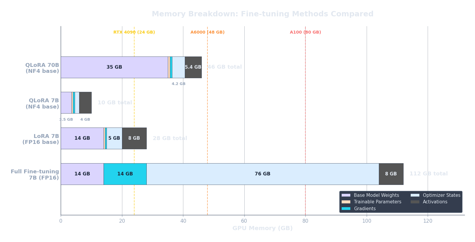

Memory is the most visible cost of full fine-tuning, but it's not the only one. Even if you have enough GPU memory to fit all the weights, gradients, and optimiser states, there's a subtler problem: updating every parameter means every parameter can drift away from its pre-trained value. What happens to the model's general capabilities when all those weights move?

Catastrophic Forgetting

Suppose you fine-tune a general-purpose model on medical question-answering. It gets great at medicine — but now it can't write Python code anymore. You didn't touch the code data, and you didn't ask it to forget. So what happened?

This phenomenon is called catastrophic forgetting (French, 1999) : when fine-tuning on task B causes the model to degrade on task A. It's one of the oldest and most stubborn problems in neural network research. The mechanism is straightforward: gradient updates push the weights toward the fine-tuning distribution and away from everything else . The model doesn't selectively update only the parameters responsible for the new task — it updates all of them, and the parameters that encoded general capabilities get overwritten in the process.

Geometrically, think of the loss landscape as a high-dimensional surface with many valleys. Pre-training found a valley that works well for many tasks simultaneously. Fine-tuning pushes the weights into a narrower valley that works brilliantly for the fine-tuning task but may be far from the valleys that served other tasks. The more steps we take (and the larger the steps), the further we drift from the general-purpose minimum.

There are several practical strategies to mitigate forgetting:

• Low learning rate: nudge, don't overwrite. Pre-training typically uses learning rates around $10^{-3}$. For fine-tuning, $10^{-5}$ to $5 \times 10^{-5}$ is standard. The smaller the steps, the closer we stay to the pre-trained valley.
• Short training: 1–3 epochs is often enough. Each additional epoch pushes the weights further toward the fine-tuning distribution. More epochs means more forgetting — there's a direct tradeoff between task-specific performance and general capability retention.
• Data mixing: include a fraction of pre-training data (or a diverse proxy) in the fine-tuning mix. This gives the model a continuous reminder of its general capabilities. Many production fine-tuning recipes mix 5–10% general data alongside the task data.
• Regularisation: explicitly penalise the weights for drifting too far from $\theta_0$. This is the idea behind Elastic Weight Consolidation (EWC) (Kirkpatrick et al., 2017) and simpler L2 penalties.

The regularisation idea can be expressed formally. Instead of minimising just the task loss, we add a penalty that grows as the weights move away from their pre-trained values:

Here $\mathcal{L}_{\text{task}}$ is the standard training loss ( cross-entropy for language modelling, for example). $\theta$ is the current set of weights and $\theta_0$ is the pre-trained starting point. The term $\|\theta - \theta_0\|^2$ is the squared L2 distance between the current and original weights — it measures how far we've drifted. And $\lambda$ is a hyperparameter that controls the strength of the penalty.

Let's check the boundaries. If $\lambda = 0$, the penalty disappears entirely and we get pure fine-tuning — the weights are free to move wherever the task loss gradient takes them. If $\lambda \to \infty$, the penalty dominates the loss and the weights effectively cannot change at all — no learning happens because any deviation from $\theta_0$ is infinitely penalised. In practice, $\lambda$ is set somewhere in between: strong enough to prevent wild drift, weak enough to allow genuine task adaptation.

Learning Rate: The Most Important Hyperparameter

If full fine-tuning is all about moving pre-trained weights toward a new task, the learning rate decides how far each step moves them. Get it wrong and one of two things happens: too high and you jump out of the good region the pre-trained model found (catastrophic forgetting, divergence, loss spikes); too low and you barely move at all (wasted compute, underfitting). For fine-tuning, the learning rate matters more than almost any other hyperparameter, because the starting point already encodes valuable structure that a careless step size can destroy.

Why is the fine-tuning learning rate so much smaller than the pre-training one? During pre-training, the model starts from random weights and needs to traverse large distances across the loss landscape to find a good region. Learning rates of $10^{-3}$ to $10^{-4}$ are typical. But at fine-tuning time, we're already in a good region. We just need to make small adjustments. A rule of thumb: start 10–100x lower than the pre-training learning rate. For most LLM fine-tuning, this means $10^{-5}$ to $5 \times 10^{-5}$.

Beyond the peak value, the schedule — how the learning rate changes over the course of training — also matters. Two schedules dominate fine-tuning:

• Linear warmup + cosine decay: the learning rate ramps up linearly from near-zero to the peak over a warmup period (typically 3–10% of total steps), then follows a cosine curve back down to near-zero. The warmup prevents early instability when gradients are noisy, and the cosine decay provides a smooth annealing. This is the standard schedule for supervised fine-tuning (SFT) of LLMs.
• Constant with warmup: ramp up linearly, then hold at the peak value for the rest of training. Simpler to implement, fewer hyperparameters (no need to tune the decay shape), and works surprisingly well for short fine-tuning runs where cosine decay barely has time to kick in.

There's a more sophisticated approach: discriminative learning rates (Howard & Ruder, 2018) . The insight is that different layers learn different kinds of features. Early layers capture general features (syntax, morphology) that transfer well across tasks and shouldn't change much. Later layers capture task-specific features and should be free to adapt more aggressively. So instead of a single learning rate, we assign a lower rate to early layers and a higher one to later layers. In ULMFiT, each layer group's rate was scaled by a factor $\xi^{-l}$ where $l$ is the layer depth (0 = last layer) and $\xi > 1$ (typically 2.6), so the earliest layers trained at a rate roughly $\xi^{-L}$ times smaller than the last layer.

The code below plots a cosine-decay schedule with linear warmup, which is the most widely used schedule for LLM fine-tuning. Notice how the learning rate rises quickly during warmup and then smoothly decays, spending most of training at moderate values rather than at the peak.

import math, json, js

total_steps = 1000
warmup_steps = 100
peak_lr = 2e-5
min_lr = 1e-6

# Compute LR at each step
steps = list(range(total_steps))
lrs_cosine = []
lrs_constant = []

for step in steps:
    # -- Cosine with warmup --
    if step < warmup_steps:
        lr = peak_lr * (step / warmup_steps)
    else:
        progress = (step - warmup_steps) / (total_steps - warmup_steps)
        lr = min_lr + 0.5 * (peak_lr - min_lr) * (1 + math.cos(math.pi * progress))
    lrs_cosine.append(lr)

    # -- Constant with warmup --
    if step < warmup_steps:
        lr_const = peak_lr * (step / warmup_steps)
    else:
        lr_const = peak_lr
    lrs_constant.append(lr_const)

# Sample every 10 steps for plotting
sample = list(range(0, total_steps, 10))
x_data = [str(s) for s in sample]

plot_data = [
    {
        "title": "Learning Rate Schedules for Fine-tuning",
        "x_label": "Training Step",
        "y_label": "Learning Rate",
        "x_data": x_data,
        "lines": [
            {
                "label": "Cosine + Warmup",
                "data": [lrs_cosine[s] for s in sample],
                "color": "#3b82f6"
            },
            {
                "label": "Constant + Warmup",
                "data": [lrs_constant[s] for s in sample],
                "color": "#f59e0b"
            }
        ]
    }
]

js.window.py_plot_data = json.dumps(plot_data)

When Full Fine-tuning Still Wins

Given the memory costs and the forgetting risks, you might wonder why anyone still does full fine-tuning. The answer is that there are real scenarios where it remains the best option — and recognising them saves you from applying parameter-efficient methods where they aren't needed.

• Small models (< 1B parameters): a 350M-parameter model needs only $16 \times 350 \times 10^6 \approx 5.6$ GB for full fine-tuning. That fits comfortably on a single consumer GPU. The overhead of setting up LoRA adapters, choosing ranks, and managing adapter files simply isn't worth it at this scale.
• Maximum quality: full fine-tuning has a slight but consistent edge over parameter-efficient methods on many benchmarks. The LoRA paper itself (Hu et al., 2021) reports that full fine-tuning matches or slightly outperforms LoRA, especially at higher ranks. When you need every fraction of a percent of accuracy — medical diagnosis, safety-critical systems — that edge can justify the extra compute.
• Single-task deployment: if you're deploying one model for one task, there's no adapter management complexity. No merging, no switching, no adapter composition. The model is the model. In production, simplicity has real value.
• When hardware is abundant: if you have access to a cluster of 8x A100s (or better), the memory wall stops being a wall. Multi-GPU training with ZeRO-3 (Rajbhandari et al., 2020) shards the optimiser state, gradients, and weights across GPUs, so the per-GPU memory cost drops roughly linearly with the number of GPUs. At that point, full fine-tuning is just as practical as LoRA — and slightly higher quality.

The decision tree is straightforward: if your model fits in memory and you can afford the compute, full fine-tuning is the safest default. It's the simplest pipeline (no adapter hyperparameters to tune) and it gives the best results. The complexity of parameter-efficient methods is only justified when memory or compute force your hand.

But what if you don't have 8x A100s? What if you want to fine-tune a 70B model on a single GPU? What if you need to serve dozens of task-specific variants from one base model without multiplying your GPU fleet? The next article introduces LoRA (Low-Rank Adaptation) — a method that freezes the pre-trained weights entirely and trains only small, low-rank matrices injected alongside each layer. It slashes the memory cost by orders of magnitude while preserving most of the quality of full fine-tuning.

Quiz

Test your understanding of full fine-tuning, its costs, and its tradeoffs.