Position Encodings for Long Context

Why Position Matters

Transformers process all tokens in parallel. Unlike RNNs, which read one token at a time and implicitly know order because token 5 is processed after token 4, a transformer's self-attention computes attention scores between every pair of tokens simultaneously. That parallelism is what makes transformers fast to train on GPUs, but it comes with a cost: the model has no inherent notion of position. Without position information, "the cat sat on the mat" and "the mat sat on the cat" produce identical attention patterns and identical outputs, because the set of tokens is the same.

The original transformer (Vaswani et al., 2017) solved this with sinusoidal positional embeddings : fixed vectors added to the token embeddings before attention, using sine and cosine functions at different frequencies to give each position a unique signature. These work well for short sequences, but they are absolute — each position gets a fixed vector regardless of context — and they don't extrapolate: a model trained on sequences of length 512 has never seen the sinusoidal pattern for position 513, so performance degrades at longer lengths.

The question driving this article is: how do we encode position so that a model can handle sequences much longer than it was trained on? Two families of modern approaches dominate:

• RoPE (Rotary Position Embedding): encodes relative position by rotating query and key vectors. Used by LLaMA, Mistral, Qwen, Gemma, and most modern open-weight LLMs.
• ALiBi (Attention with Linear Biases): adds a simple linear penalty to attention scores based on token distance. No learned positional parameters at all. Used by BLOOM and MPT.

We will build up from the basic RoPE formulation, explain why it encodes relative position, then cover ALiBi as a radical alternative, and finally show how RoPE can be extended beyond its training length with NTK-aware scaling and YaRN.

RoPE: Rotary Position Embedding

RoPE (Su et al., 2021) encodes position by rotating query and key vectors in 2D subspaces. The core idea is beautifully geometric: instead of adding a position vector to the embedding (which mixes position and content), RoPE applies a rotation that depends on position. When we compute the dot product between a rotated query and a rotated key, the rotation angles compose in a way that depends only on the relative distance between the two positions, not their absolute values.

Here is how it works. Given a $d$-dimensional vector $\mathbf{x}$ at position $m$, split it into $d/2$ consecutive pairs: $(x_0, x_1), (x_2, x_3), \ldots, (x_{d-2}, x_{d-1})$. Each pair $i$ is treated as a 2D vector (or equivalently, a complex number $x_{2i} + ix_{2i+1}$ — see the Euler's formula article for why this works) and rotated by the angle $m \cdot \theta_i$:

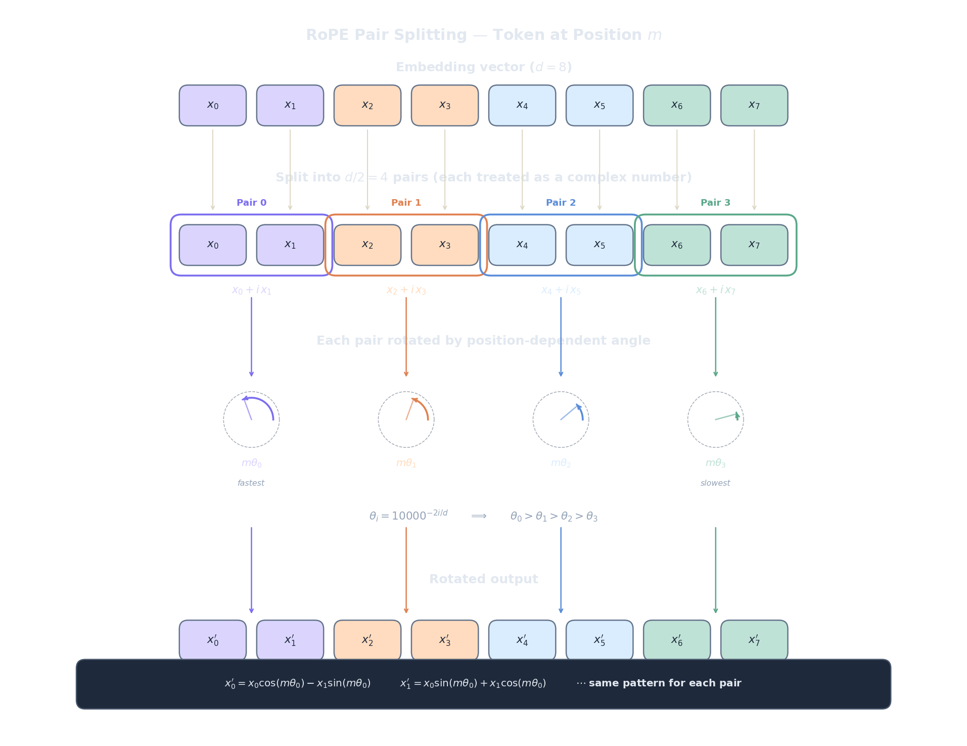
where the frequency for dimension pair $i$ is:

Let's unpack every piece of this formula:

• $m$ is the position index (0, 1, 2, ...). It tells us where the token sits in the sequence.
• $\theta_i$ is the rotation frequency for dimension pair $i$. It controls how fast the rotation angle grows with position.
• $m \cdot \theta_i$ is the actual rotation angle in radians. Position $m$ in dimension pair $i$ gets rotated by this amount.
• The $\cos / \sin$ structure is a standard 2D rotation matrix applied to the pair $(x_{2i}, x_{2i+1})$. This is the same rotation you'd use to turn a 2D point by an angle.

Now the boundary analysis for $\theta_i = 10000^{-2i/d}$. When $i = 0$ (the first dimension pair), $\theta_0 = 10000^0 = 1$, which is the highest frequency — the rotation angle grows by 1 radian per position, cycling rapidly. This encodes fine-grained local position: neighbouring tokens get very different rotation angles. When $i = d/2 - 1$ (the last dimension pair), $\theta_{d/2-1} = 10000^{-1} \approx 0.0001$, an extremely low frequency — the rotation angle barely changes between adjacent positions. This encodes coarse global position: tokens far apart are distinguishable, but neighbours look nearly identical. The analogy is a positional number system: low-frequency dimensions are the "high-order digits" (like the hundreds place), and high-frequency dimensions are the "low-order digits" (like the ones place).

Now the critical property that makes RoPE a relative position encoding. When we compute the dot product between a query at position $m$ and a key at position $n$, each dimension pair contributes:

The key insight is that this simplifies because rotating by angle $\alpha$ then taking the dot product with something rotated by angle $\beta$ is equivalent to the unrotated dot product of one vector with the other rotated by $\alpha - \beta$. In matrix form, $R(m)^\top R(n) = R(m - n)$, where $R(\cdot)$ is the block-diagonal rotation matrix. The dot product depends only on the relative position $m - n$ , not on the absolute positions $m$ and $n$ individually. Token 5 attending to token 3 produces the same positional signal as token 105 attending to token 103.

This is why RoPE has become dominant: it provides relative position information injected directly into the attention dot product, requires zero additional parameters, and composes cleanly with the standard QKV attention mechanism. It is used by LLaMA , Mistral , Qwen , Gemma , and virtually every modern open-weight LLM.

The plot below visualises the rotation angles $m \cdot \theta_i$ for different positions and dimension pairs. Notice how the first pairs (low $i$, high frequency) cycle rapidly while the last pairs (high $i$, low frequency) change very slowly.

import math, json, js

d = 64  # embedding dimension
n_pairs = d // 2  # 32 dimension pairs
positions = list(range(128))  # positions 0..127

# Compute theta_i for selected dimension pairs
selected_pairs = [0, 4, 12, 24, 31]  # low i = high freq, high i = low freq
pair_labels = [f"pair i={i} (theta={10000**(-2*i/d):.4f})" for i in selected_pairs]

lines = []
colors = ["#ef4444", "#f59e0b", "#22c55e", "#3b82f6", "#8b5cf6"]
for idx, i in enumerate(selected_pairs):
    theta_i = 10000 ** (-2 * i / d)
    # Compute rotation angle mod 2*pi for visualisation
    angles = [(m * theta_i) % (2 * math.pi) for m in positions]
    lines.append({
        "label": pair_labels[idx],
        "data": [round(a, 4) for a in angles],
        "color": colors[idx]
    })

plot_data = [
    {
        "title": "RoPE Rotation Angles (mod 2pi) by Position",
        "x_label": "Position m",
        "y_label": "Angle (radians)",
        "x_data": [str(p) for p in positions],
        "lines": lines
    }
]
js.window.py_plot_data = json.dumps(plot_data)
print("Low i (red) = high frequency: angle cycles rapidly with position.")
print("High i (purple) = low frequency: angle barely changes between neighbours.")
print("This multi-scale encoding lets RoPE distinguish both nearby and distant tokens.")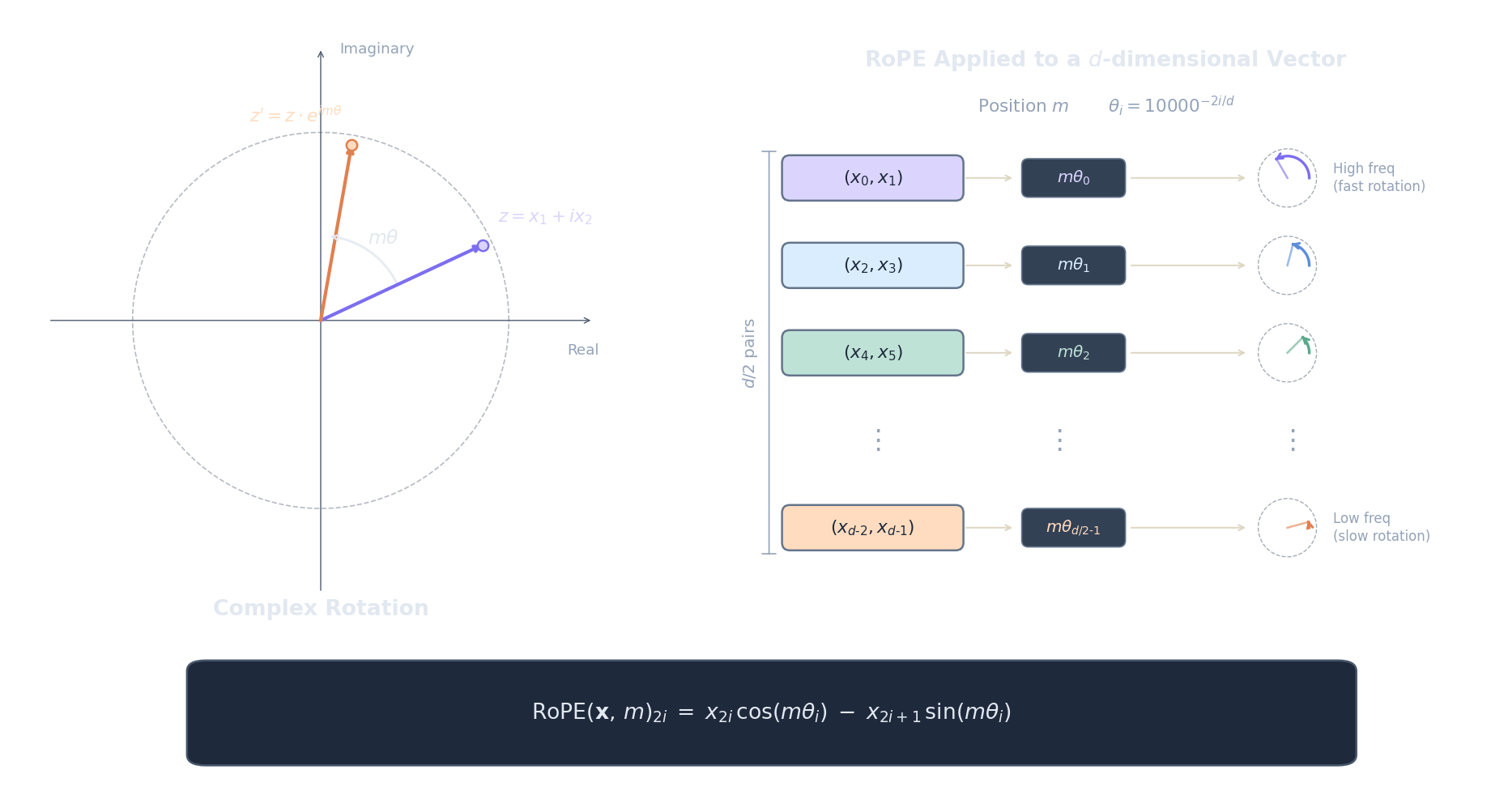

The code below implements RoPE on a small vector and demonstrates the relative-position property: the dot product between a rotated query at position $m$ and a rotated key at position $n$ depends only on $m - n$.

import math, json, js

def rope(x, m, d):
    """Apply RoPE rotation to vector x at position m."""
    out = list(x)
    for i in range(d // 2):
        theta_i = 10000 ** (-2 * i / d)
        angle = m * theta_i
        cos_a, sin_a = math.cos(angle), math.sin(angle)
        x0, x1 = x[2*i], x[2*i+1]
        out[2*i]   = x0 * cos_a - x1 * sin_a
        out[2*i+1] = x0 * sin_a + x1 * cos_a
    return out

def dot(a, b):
    return sum(ai * bi for ai, bi in zip(a, b))

d = 8
# Fixed query and key vectors (content, before rotation)
q = [0.5, -0.3, 0.8, 0.1, -0.6, 0.4, 0.2, -0.7]
k = [0.3, 0.6, -0.2, 0.5, 0.7, -0.1, 0.4, 0.3]

# Compute dot products for various (m, n) pairs with same m-n
rows = []
for m, n in [(5, 3), (10, 8), (50, 48), (100, 98), (1000, 998)]:
    q_rot = rope(q, m, d)
    k_rot = rope(k, n, d)
    dp = dot(q_rot, k_rot)
    rows.append([str(m), str(n), str(m - n), f"{dp:.6f}"])

# Also show a different relative distance for contrast
for m, n in [(5, 2), (10, 7), (100, 97)]:
    q_rot = rope(q, m, d)
    k_rot = rope(k, n, d)
    dp = dot(q_rot, k_rot)
    rows.append([str(m), str(n), str(m - n), f"{dp:.6f}"])

js.window.py_table_data = json.dumps({
    "headers": ["Query pos m", "Key pos n", "m - n", "Dot product"],
    "rows": rows
})
print("All rows with m-n=2 have the SAME dot product regardless of absolute position.")
print("All rows with m-n=3 have a DIFFERENT (but consistent) dot product.")
print("This confirms RoPE encodes relative, not absolute, position.")

ALiBi: No Embeddings, Just Bias

ALiBi (Press et al., 2022) takes a radically different approach: remove all positional embeddings entirely . No sinusoidal vectors, no rotations, no learned position parameters. Instead, ALiBi adds a simple linear bias directly to the attention scores that penalises distant tokens:

where $m$ is a head-specific slope . That's the entire method: subtract a penalty proportional to the distance between query position $i$ and key position $j$. Nearby tokens get a small penalty, distant tokens get a large one, and after softmax, this translates to a recency bias: the model naturally attends more to nearby tokens.

The slopes are fixed (not learned) and form a geometric sequence across the $H$ attention heads:

for head $h = 1, 2, \ldots, H$. Different heads get different slopes, which means different heads specialise in different attention ranges:

• Small $m$ (early heads): gentle decay. A token 100 positions away loses only a few points. These heads can attend broadly across the entire context.
• Large $m$ (later heads): steep decay. Even tokens 10 positions away get heavily penalised. These heads focus on local context.

Boundary analysis: if $m = 0$, there is no positional bias at all — the model attends uniformly based on content alone, like a transformer with no positional encoding. As $m \to \infty$, the penalty for any non-zero distance becomes infinite, so the model can only attend to the current token (position $i = j$). The geometric sequence of slopes provides a smooth spectrum between these extremes.

Why does ALiBi extrapolate so well? The linear bias is a simple inductive prior: "recent tokens are more likely to be relevant." Because it's additive to the raw attention logits (not a learned embedding tied to specific position indices), there's nothing that breaks at unseen positions. Position 2048 gets a penalty of $m \cdot 2048$ relative to the current token, which is just a larger version of the same linear function the model saw during training. There are zero learned positional parameters.

The code below shows how ALiBi slopes are assigned across heads, and what the attention bias matrix looks like for a short sequence.

import math, json, js

H = 8  # number of attention heads
seq_len = 6

# Compute ALiBi slopes: m_h = 2^(-8h/H) for h=1..H
slopes = [2 ** (-8 * h / H) for h in range(1, H + 1)]

rows_slopes = []
for h in range(H):
    rows_slopes.append([
        f"Head {h+1}",
        f"{slopes[h]:.6f}",
        "Broad (global)" if slopes[h] < 0.01 else "Narrow (local)" if slopes[h] > 0.1 else "Medium"
    ])

js.window.py_table_data = json.dumps({
    "headers": ["Head", "Slope m", "Attention Range"],
    "rows": rows_slopes
})

# Show bias matrix for head 1 (smallest slope) and head 8 (largest slope)
print(f"Slopes range from {slopes[0]:.6f} (head 1, broadest) to {slopes[-1]:.6f} (head {H}, narrowest)")
print(f"Head 1 penalty for distance 100: {slopes[0] * 100:.2f}")
print(f"Head {H} penalty for distance 100: {slopes[-1] * 100:.1f}")
print(f"Head 1 barely penalises distant tokens; Head {H} makes them nearly invisible after softmax.")

ALiBi is used by BLOOM (BigScience, 176B parameters) and MPT (MosaicML). However, despite its elegance, most newer models have converged on RoPE instead. One reason is that ALiBi's strict linear decay can be too aggressive for tasks requiring long-range dependencies: the attention to distant tokens is suppressed by design, which helps extrapolation but can hurt when the model genuinely needs information from 1000 tokens ago.

Extending RoPE: NTK-Aware Scaling and YaRN

RoPE doesn't extrapolate well out of the box. If a model was trained with a maximum sequence length $L = 4096$, what happens at position $m = 5000$? The rotation angles $m \cdot \theta_i$ reach values the model never saw during training. For high-frequency dimension pairs, the angles wrap around (which is fine, since the model saw all phases). But for low-frequency pairs, the angles enter an entirely new range, and the model produces degraded attention patterns.

Several methods address this by modifying how positions or frequencies are scaled.

Linear scaling (used by Meta for Code Llama) is the simplest approach. To extend from training length $L$ to target length $L'$, divide all positions by a scale factor $s = L'/L$:

This maps the extended range $[0, L']$ back into $[0, L]$, so the model only sees rotation angles it encountered during training. But there's a cost: all frequencies are compressed by the same factor, and the high-frequency dimensions (which encode fine-grained local position) lose resolution. Tokens that were previously distinguishable (positions 10 and 11) now map to positions that are only $1/s$ apart, making it harder for the model to distinguish neighbours.

NTK-aware scaling (bloc97, 2023) takes a smarter approach. Instead of scaling positions (which hurts all frequencies equally), it changes the base frequency :

where $b = 10000$ is the original base and $\alpha$ depends on the extension ratio $L'/L$. The key insight is that this modifies different frequency bands differently. Recall the number-system analogy: RoPE dimensions are like digits in a positional number system. Low-frequency dimensions are the "high-order digits" (coarse position: which thousands-of-tokens block are we in?), and high-frequency dimensions are the "low-order digits" (fine position: which specific token within a local window?).

When we increase the base, the low-frequency components (which are already close to $10000^{-1}$) get further compressed — their range is extended to cover the longer sequence. But the high-frequency components (close to $10000^0 = 1$) are barely affected, preserving the model's ability to distinguish adjacent tokens. It's like extending a number system's range (adding more "high-order digits") without touching the least-significant digits. This is much better than linear scaling, which blurs the fine-grained digits too.

YaRN (Peng et al., 2023) refines this further with three innovations:

• NTK-by-parts interpolation: instead of applying one scaling factor to all dimensions, YaRN splits them into three groups. Low-frequency dimensions (high-order digits) get interpolated, because they need to cover a wider range. High-frequency dimensions (low-order digits) are kept unchanged, because they already work fine for local position. Medium-frequency dimensions get a smooth ramp between the two treatments.
• Attention temperature correction: extending context changes the distribution of attention logits (more tokens means the softmax becomes flatter). YaRN compensates with a temperature factor:

where $s$ is the scale factor. When $s = 1$ (no extension), $t = 1$ and attention is unchanged. As $s$ grows, $t$ increases slightly, sharpening the softmax to compensate for the larger number of positions competing for attention mass. At $s = 4\times$ extension, $t \approx 1.14$; at $s = 16\times$, $t \approx 1.28$. The logarithmic growth means the correction is gentle and doesn't overcorrect.

The result: YaRN can extend a model's context length by 4-16x with only around 400 steps of fine-tuning (compared to the millions of steps in the original pretraining). Many open-source long-context models use YaRN or closely related variants. LLaMA 3's context extension, for example, uses a technique in the same family — different per-dimension treatment of RoPE frequencies combined with a modest amount of continued training.

Comparing Position Encodings

The table below summarises the position encoding methods we have covered. The field has largely converged on RoPE plus some form of frequency scaling for most production LLMs. ALiBi remains an interesting alternative with zero learned parameters, but adoption has slowed. Sinusoidal embeddings are considered legacy for decoder-only models, though they are still used in some encoder architectures.

import json, js

rows = [
    ["Sinusoidal (Vaswani 2017)", "0", "Absolute", "Poor", "Original Transformer", "Fixed sin/cos added to embeddings"],
    ["Learned Absolute", "L * d", "Absolute", "None", "GPT-2, BERT", "Lookup table per position"],
    ["RoPE (Su 2021)", "0", "Relative (via rotation)", "Poor without scaling", "LLaMA, Mistral, Qwen, Gemma", "Rotates Q,K in 2D subspaces"],
    ["ALiBi (Press 2022)", "0", "Relative (via bias)", "Good (native)", "BLOOM, MPT", "Linear penalty on distance"],
    ["RoPE + Linear Scaling", "0", "Relative", "Moderate", "Code Llama", "Divide positions by scale factor"],
    ["RoPE + NTK-aware", "0", "Relative", "Good", "Various open-source", "Scale the base frequency"],
    ["RoPE + YaRN (Peng 2023)", "0 + temp", "Relative", "Excellent", "Many long-context models", "Per-band scaling + temperature"],
]

js.window.py_table_data = json.dumps({
    "headers": ["Method", "Learned Params", "Type", "Extrapolation", "Used By", "Key Idea"],
    "rows": rows
})

print("The trend is clear: the field moved from absolute to relative encodings,")
print("and from fixed methods to ones that can be extended post-training.")
print("RoPE + scaling variants dominate modern LLMs.")

One pattern stands out: every successful method either encodes relative position (RoPE, ALiBi) or can be adapted to handle positions beyond training length (the scaling variants). Absolute encodings (sinusoidal, learned) are fundamentally limited because they tie each position to a fixed representation, making extrapolation impossible without modifications.

Quiz

Test your understanding of position encodings for long context.