Position, Residuals, and the Feed-Forward Block

Why Doesn't Attention Know About Word Order?

Multi-head attention gives us a powerful way for tokens to communicate, but there is something conspicuously absent from the mechanism. If we take a sentence and shuffle the token order, the attention output for each token changes (because the values it averages over have moved), but the attention weights between any two tokens remain identical. That's because the dot product $q_i^\top k_j$ depends only on the content of tokens $i$ and $j$, not on where they sit in the sequence. Attention is permutation-equivariant : permuting the input rows permutes the output rows in the same way, without the mechanism itself ever knowing that a permutation happened.

This is a problem because word order carries enormous meaning. "The dog bit the man" and "The man bit the dog" contain the same words, but mean very different things. If we feed both sentences through attention without any positional signal, the model has no way to distinguish between them (since every token-to-token score depends only on what the tokens are, not where they appear).

The solution from (Vaswani et al., 2017) is to add a positional encoding to each token's embedding before it enters the first attention layer. This encoding is a vector of the same dimension $d_{\text{model}}$ that depends only on the token's position in the sequence. By adding it to the content embedding, we fuse "what this token is" with "where this token sits," and all subsequent attention computations can use both signals.

The original transformer uses a deterministic encoding based on sinusoidal functions. For position $\text{pos}$ and dimension $i$, the encoding alternates between sine and cosine at exponentially increasing wavelengths.

This formula looks dense, but the intuition becomes clear when we examine what happens at different dimensions. The denominator $10000^{2i/d_{\text{model}}}$ controls the wavelength: when $i = 0$ (the first pair of dimensions), the denominator is $10000^0 = 1$, so the sine and cosine oscillate at the fastest rate (one full cycle per $2\pi \approx 6.28$ positions). When $i$ approaches $d_{\text{model}}/2$ (the last pair), the denominator grows to $10000$, so the wave stretches over roughly 62,832 positions before completing a cycle. This gives us a spectrum ranging from high-frequency waves that distinguish adjacent tokens to low-frequency waves that distinguish tokens thousands of positions apart.

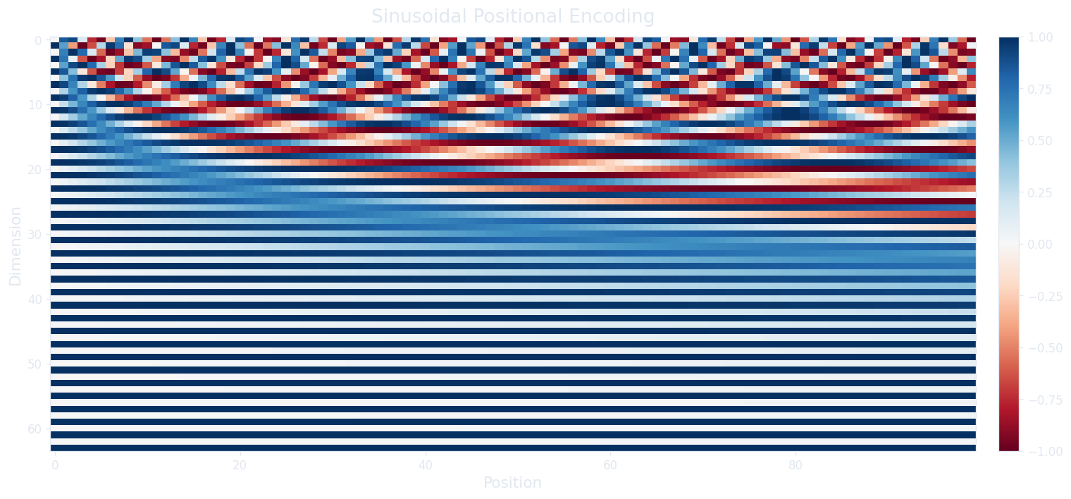
Why alternating sine and cosine? Because for any fixed offset $k$, the encoding at position $\text{pos} + k$ can be written as a linear combination of the encoding at position $\text{pos}$. This property (which follows from the trigonometric identity $\sin(\alpha + \beta) = \sin\alpha \cos\beta + \cos\alpha \sin\beta$) means the model can learn to attend to relative positions through linear transformations of the queries and keys. If we had used only sine (or only cosine), we would lose this: a single sinusoid at a given frequency doesn't let us uniquely recover the offset through a linear operation.

How Do Deep Transformers Avoid Vanishing Gradients?

We now have a multi-head attention layer enriched with positional information. A natural next step is to stack many of these layers to build a deep model, since deeper networks tend to learn richer representations. But stacking layers naively creates a well-known problem: during backpropagation, the gradient must flow through every layer's transformation, and each layer's Jacobian multiplies into the chain. If those Jacobians consistently have eigenvalues less than 1, the gradient shrinks exponentially with depth and the early layers stop learning. This is the vanishing gradient problem , and it plagued deep networks long before transformers.

The solution, borrowed from ResNets (He et al., 2015) , is a residual connection : instead of computing $\text{output} = f(x)$, we compute $\text{output} = x + f(x)$. The gradient of $x + f(x)$ with respect to $x$ is $I + \frac{\partial f}{\partial x}$, where $I$ is the identity. Even if $\frac{\partial f}{\partial x}$ is small, the identity term guarantees a gradient of at least 1 flowing straight through. This creates what we can think of as a "gradient highway" that bypasses the layer's transformation entirely, allowing the signal to reach early layers without attenuation.

There is also an elegant framing of what this means for learning. Without the residual connection, each layer must learn the full transformation from input to desired output. With the residual connection, each layer only needs to learn the residual (the delta, the correction, the difference between the input and the desired output). If the optimal function is close to the identity (which it often is in deeper layers, where representations have already been refined), the layer can learn to output near-zero, effectively passing the input through unchanged. Learning "do almost nothing" is much easier for a neural network than learning a full identity mapping, and this makes optimization smoother across many layers.

In the transformer, residual connections wrap both the attention sublayer and the feed-forward sublayer. Each block takes its input, processes it through the sublayer, and adds the result back to the original input.

Where Does Layer Normalization Fit In?

Residual connections solve the gradient flow problem, but they introduce another issue: since each layer adds its output to the running sum, the magnitude of the activations can grow with depth. After 12 layers of additions, the hidden states might have much larger norms than the initial embeddings, and this scale drift can destabilize training (large activations lead to large gradients, which lead to large weight updates, which lead to even larger activations).

Layer normalization (Ba et al., 2016) addresses this by normalizing the activations within each token's representation. For a vector $\mathbf{x}$ of dimension $d_{\text{model}}$, we compute the mean $\mu$ and variance $\sigma^2$ across the dimensions, normalize, and apply learnable scale ($\gamma$) and shift ($\beta$) parameters.

The $\epsilon$ term (typically $10^{-5}$) prevents division by zero when the variance is very small, and the learnable $\gamma$ and $\beta$ allow the model to undo the normalization if that turns out to be useful (they give the layer the expressiveness to learn the identity function through the normalization if needed).

An important architectural choice is where to place the normalization relative to the sublayer. The original transformer paper (Vaswani et al., 2017) used post-norm : first compute the sublayer, add the residual, then normalize. This means the normalization acts on the sum $x + \text{Sublayer}(x)$.

Most modern transformers (GPT-2, GPT-3, LLaMA, and many others) use pre-norm instead: normalize first, then apply the sublayer, then add the residual. Xiong et al. (2020) ("On Layer Normalization in the Transformer Architecture") showed that pre-norm tends to produce more stable gradients at initialization, which makes training easier (especially for deeper models) and often removes the need for a careful learning rate warmup schedule.

Why Does the Transformer Need a Feed-Forward Network?

At this point we have attention (enriched with positional information), residual connections, and layer normalization. If we stacked only attention layers, would that be enough? Attention lets tokens gather information from other tokens, but there is no mechanism for a token to transform its own representation through a non-linear function after it has collected that information. Every step so far has been either a linear projection or a softmax-weighted average, and stacking linear operations produces another linear operation. Without a non-linearity, the network's expressiveness would plateau regardless of depth.

The position-wise feed-forward network (FFN) fills this gap. It consists of two linear transformations with a non-linearity between them, applied independently to each token.

Here $W_1$ has shape $(d_{\text{model}}, d_{\text{ff}})$ and $W_2$ has shape $(d_{\text{ff}}, d_{\text{model}})$, where $d_{\text{ff}}$ is typically $4 \times d_{\text{model}}$. The original paper used ReLU as $\sigma$; many modern models use GELU (Hendrycks & Gimpel, 2016) or SwiGLU (Shazeer, 2020) instead, which tend to train more smoothly.

Let's walk through the shapes to understand the expansion and compression. If $d_{\text{model}} = 512$ and $d_{\text{ff}} = 2048$, then $W_1$ projects each token from 512 dimensions to 2048 (expanding the representation by 4x), the non-linearity is applied element-wise, and $W_2$ projects back down from 2048 to 512. This bottleneck architecture (expand, transform, compress) gives the network a high-dimensional space in which to perform non-linear computation, then compresses the result back to $d_{\text{model}}$ so it can be fed to the next layer.

What would break if we removed $\sigma$? Without the non-linearity, $W_2 (W_1 x + b_1) + b_2$ collapses to a single affine transformation $Ax + b$ (since the composition of two linear maps is linear). Two layers of parameters would offer no more expressive power than one. The non-linearity is what allows the FFN to learn functions that attention alone cannot represent. And if $d_{\text{ff}}$ were equal to $d_{\text{model}}$ instead of $4 \times d_{\text{model}}$? The network could still apply non-linear transformations, but in a lower-dimensional space, limiting the variety of features it can extract. Empirically, the 4x expansion strikes a balance between capacity and parameter count; smaller ratios tend to hurt performance while larger ones show diminishing returns.

There is a key architectural distinction between attention and the FFN that is worth emphasizing. Attention is a communication mechanism: it moves information between tokens (or, in graph terms, it passes messages between nodes). The FFN is a computation mechanism: it transforms each token's representation independently, with no interaction between positions. This means the FFN at position 5 has no idea what the token at position 3 looks like (it processes the vector at position 5 in complete isolation). All inter-token information exchange must happen through attention; the FFN's job is to process what attention gathered.

Recent work has suggested that the FFN layers act as a form of key-value memory, where $W_1$ stores learned patterns (keys) and $W_2$ stores the associated output (values). Geva et al. (2021) ("Transformer Feed-Forward Layers Are Key-Value Memories") showed that individual neurons in the first layer often activate for interpretable input patterns (specific words, syntactic structures, or semantic categories), and the corresponding columns of $W_2$ tend to promote predictable next-token distributions. In this view, the FFN is where the transformer stores factual knowledge, while attention is how it routes and composes that knowledge.

What Does a Complete Transformer Block Look Like?

We can now assemble all the pieces into a single transformer block. Each block applies two sublayers (multi-head attention and a feed-forward network), each wrapped in a residual connection and layer normalization. Using pre-norm ordering (the modern convention), a block takes input $x$ and produces output $x'$ as follows.

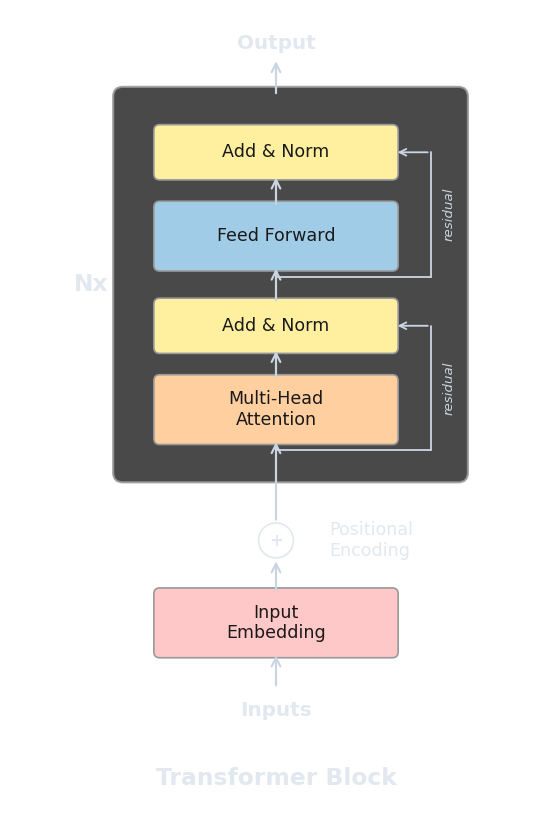
The following implementation puts all of our components together into a complete pre-norm transformer block, including the multi-head attention class from the previous article.

import torch
import torch.nn as nn
import torch.nn.functional as F

class MultiHeadAttention(nn.Module):
    def __init__(self, d_model, num_heads):
        super().__init__()
        self.num_heads = num_heads
        self.d_k = d_model // num_heads
        self.W_Q = nn.Linear(d_model, d_model, bias=False)
        self.W_K = nn.Linear(d_model, d_model, bias=False)
        self.W_V = nn.Linear(d_model, d_model, bias=False)
        self.W_O = nn.Linear(d_model, d_model, bias=False)

    def forward(self, x, mask=None):
        B, T, C = x.shape
        Q = self.W_Q(x).view(B, T, self.num_heads, self.d_k).transpose(1, 2)
        K = self.W_K(x).view(B, T, self.num_heads, self.d_k).transpose(1, 2)
        V = self.W_V(x).view(B, T, self.num_heads, self.d_k).transpose(1, 2)

        scores = (Q @ K.transpose(-2, -1)) / (self.d_k ** 0.5)
        if mask is not None:
            scores = scores.masked_fill(mask == 0, float('-inf'))
        attn = F.softmax(scores, dim=-1)

        out = (attn @ V).transpose(1, 2).contiguous().view(B, T, C)
        return self.W_O(out)


class FeedForward(nn.Module):
    def __init__(self, d_model, d_ff):
        super().__init__()
        self.W1 = nn.Linear(d_model, d_ff)
        self.W2 = nn.Linear(d_ff, d_model)

    def forward(self, x):
        return self.W2(F.gelu(self.W1(x)))


class TransformerBlock(nn.Module):
    """Pre-norm transformer block: LN -> Attention -> residual -> LN -> FFN -> residual"""
    def __init__(self, d_model, num_heads, d_ff):
        super().__init__()
        self.ln1 = nn.LayerNorm(d_model)
        self.attn = MultiHeadAttention(d_model, num_heads)
        self.ln2 = nn.LayerNorm(d_model)
        self.ffn = FeedForward(d_model, d_ff)

    def forward(self, x, mask=None):
        # Sublayer 1: attention with pre-norm and residual
        x = x + self.attn(self.ln1(x), mask)
        # Sublayer 2: FFN with pre-norm and residual
        x = x + self.ffn(self.ln2(x))
        return x


# --- Verify shapes and parameter counts ---
d_model = 512
num_heads = 8
d_ff = 2048  # 4x expansion
T = 10
batch = 2

block = TransformerBlock(d_model, num_heads, d_ff)
x = torch.randn(batch, T, d_model)
out = block(x)

print(f"Input shape:  {x.shape}")
print(f"Output shape: {out.shape}")
print()

# Count parameters by component
attn_params = sum(p.numel() for p in block.attn.parameters())
ffn_params = sum(p.numel() for p in block.ffn.parameters())
ln_params = sum(p.numel() for p in block.ln1.parameters()) + \
            sum(p.numel() for p in block.ln2.parameters())
total = sum(p.numel() for p in block.parameters())

print(f"Attention params:  {attn_params:>10,}")
print(f"FFN params:        {ffn_params:>10,}")
print(f"LayerNorm params:  {ln_params:>10,}")
print(f"Total params:      {total:>10,}")
print(f"FFN share:         {ffn_params/total:.1%}")

Notice how the TransformerBlock.forward method is just four lines. The first two apply pre-norm attention with a residual connection, and the second two do the same for the FFN. This simplicity is one of the transformer's most appealing properties: every layer has exactly the same structure, the input and output shapes are identical, and stacking $N$ layers is just a loop. The entire GPT-2 architecture, for instance, is an embedding layer, 12 (or 24, or 48) copies of this block, a final layer norm, and a linear head.

The parameter counts printed above confirm our earlier observation about the FFN's dominance. With the standard $4 \times$ expansion factor, the FFN accounts for roughly two-thirds of each block's parameters, while attention accounts for about one-third. This ratio holds regardless of $d_{\text{model}}$, since both components scale as $O(d_{\text{model}}^2)$.

Quiz

Test your understanding of the components that complete the transformer block.