Dense Retrieval: From BERT to Bi-Encoders

The Dense Representation Idea

The previous article ended with a problem: BM25 can only match documents that share the exact same words as the query. Search for "cardiac arrest" and we miss every document that says "heart attack". No matter how good the scoring formula is, zero shared terms means zero score.

What if, instead of matching words, we matched meanings? The idea behind dense retrieval is to represent every document and query as a compact vector (typically 768 dimensions) where geometric proximity captures semantic similarity. Two texts that mean the same thing end up close together in this space, even if they share no words at all.

The scoring function becomes a dot product (or cosine similarity) between these vectors:

Most dense retrieval models normalise their output vectors to unit length ($\|\mathbf{e}_q\| = \|\mathbf{e}_d\| = 1$), which makes the dot product and cosine similarity identical: $\mathbf{e}_q \cdot \mathbf{e}_d = \cos \theta$. When we say "similarity" throughout this article, either metric gives the same ranking.

In this space, "cardiac arrest" and "heart attack" can have nearly identical vectors, so retrieval surfaces documents about either. The vocabulary mismatch problem from the previous article is gone. The tradeoff is that we lose the exact inverted-index lookup that made sparse methods fast, and instead need approximate nearest-neighbour search to find close vectors efficiently (covered in article 7).

BERT: The Contextual Foundation

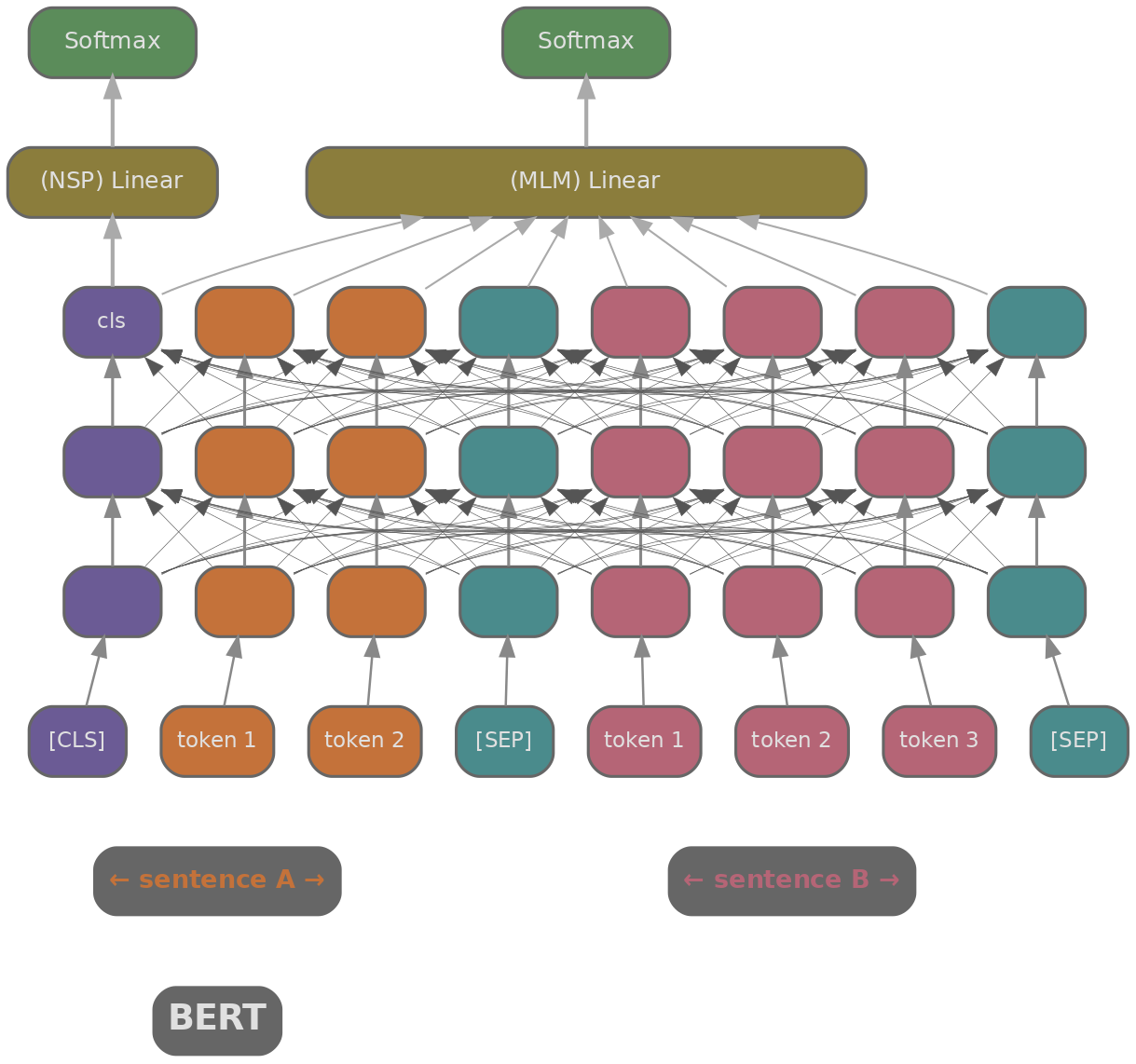
We need a way to turn text into a vector that captures its meaning. BERT (Devlin et al., 2019) (Bidirectional Encoder Representations from Transformers) was the first model to do this well. It's a transformer encoder trained with masked language modelling (MLM) and next-sentence prediction (NSP), producing contextual embeddings where each token's representation depends on the full surrounding context.

The most obvious way to use BERT for retrieval is to concatenate the query and document together: [CLS] query [SEP] document [SEP], then use the [CLS] token's output to predict relevance. This is called a cross-encoder : every query token attends to every document token through all transformer layers, so the model captures fine-grained interactions between them. On benchmarks like MS MARCO (Bajaj et al., 2016) , cross-encoders achieve excellent relevance scores.

The problem is computational. Scoring a query against 10 million documents means 10 million forward passes through BERT. At roughly 2ms per pass on a GPU, that's about 20,000 seconds per query. Cross-encoders are accurate but far too slow for first-stage retrieval.

SBERT: Encoding Query and Document Separately

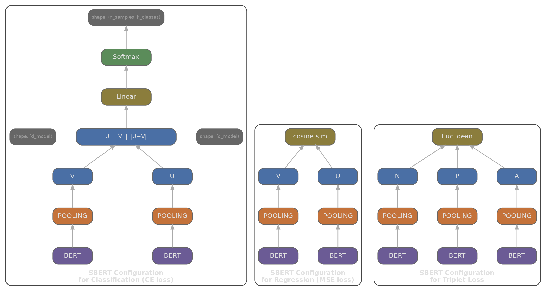
If the cross-encoder bottleneck is that query and document must be processed together, the natural fix is to encode them separately. Sentence-BERT (Reimers & Gurevych, 2019) introduced this bi-encoder architecture: two BERT models (sharing weights) each produce an embedding independently, giving the query its own vector and the document its own vector, so that retrieval reduces to a similarity computation between them.

Since document embeddings don't depend on the query, we can compute them all offline and store them in a dense index. At query time, we only run one forward pass (for the query) and then do a fast vector search against the precomputed document embeddings. Scoring a query against 10 million documents becomes a matrix multiplication instead of 10 million BERT forward passes.

To get a single vector from BERT's sequence of token embeddings, we need a pooling strategy:

• use the [CLS] token's embedding directly. Simple, but [CLS] was trained for next-sentence prediction (a coarse binary signal), not for producing a good sentence-level summary, so it tends to underperform on retrieval tasks.
• average all token embeddings (excluding padding): $\mathbf{e} = \frac{1}{|T|} \sum_{i \in T} \mathbf{h}_i$. This tends to outperform [CLS] pooling on most similarity benchmarks, likely because it incorporates signal from every token rather than relying on a single position.
• take the element-wise maximum across all token positions. Captures the strongest feature per dimension, but is less common in practice.

SBERT is trained on Natural Language Inference (NLI) datasets: sentence pairs labelled as entailment (pull together), contradiction (push apart), or neutral. This gives it a good general sense of semantic similarity, but it wasn't specifically trained for retrieval.

DPR: Training Bi-Encoders for Retrieval

SBERT knows about semantic similarity, but retrieval is a different task. "How tall is the Eiffel Tower?" and "The Eiffel Tower is 330 metres tall" aren't semantically similar in the NLI sense (one is a question, one is a statement), but the second is exactly what we want to retrieve. Dense Passage Retrieval (Karpukhin et al., 2020) (DPR) addressed this by training bi-encoders end-to-end on question-answering data: given a question, retrieve the Wikipedia passage containing the answer.

DPR uses two separate BERT encoders: one for queries, one for passages. The two encoders run independently (two separate forward passes), so queries and passages never attend to each other. Training uses a contrastive loss called InfoNCE that pushes each question's positive passage closer in embedding space while pushing negatives farther away:

Where do the negatives come from? We train on $B$ query-passage pairs per batch. Each query $q_i$ has one positive passage $p_i^+$. Since all $B$ passages are encoded in the same batch, the $B-1$ passages that belong to other queries serve as negatives for $q_i$ (they are unlikely to be relevant to $q_i$). This technique is called in-batch negatives , and it is efficient because a batch of $B$ pairs yields $B$ training examples with $B-1$ negatives each, all from forward passes we were already computing. The resulting similarity matrix is $B \times B$, the diagonal entries are positives, and the loss sums across rows. DPR also mixes in a few BM25 hard negatives per query to strengthen the training signal.

DPR showed that training specifically on retrieval data substantially outperforms using SBERT (trained for general similarity) for passage retrieval, with top-20 accuracy jumping from roughly 59% to 79% on Natural Questions (Karpukhin et al., 2020, Table 1) . This gap suggests that the optimal embedding space for retrieval is not the same as for general sentence similarity.

The simulation below shows how InfoNCE loss evolves as training progresses. We build a $B \times B$ similarity matrix at four stages (untrained, early, mid, converged) and compute the mean loss across queries. As the diagonal entries (positive pairs) begin to dominate, the loss drops.

import math, json
import js

# Simulate the in-batch negatives training signal
# For a batch of B queries, we compute a B x B similarity matrix
# Loss = NLL on the diagonal (positive pairs)

def softmax(logits):
    m = max(logits)
    exp_logits = [math.exp(x - m) for x in logits]
    s = sum(exp_logits)
    return [e / s for e in exp_logits]

def infonce_loss(sim_matrix):
    """For each query row, the diagonal entry is the positive."""
    B = len(sim_matrix)
    losses = []
    for i in range(B):
        row = sim_matrix[i]
        probs = softmax(row)
        # Loss is negative log probability of the diagonal (positive)
        losses.append(-math.log(probs[i] + 1e-9))
    return losses

# Simulate similarity matrices at different training stages
B = 6

# Early training: embeddings close to random, low contrast
def make_matrix(diag_boost, off_diag_noise, B):
    matrix = []
    for i in range(B):
        row = []
        for j in range(B):
            if i == j:
                row.append(diag_boost + (0.1 * ((i * 3 + 7) % 5 - 2)) / 10)
            else:
                row.append(off_diag_noise * ((i * 7 + j * 13 + 11) % 10 - 5) / 10)
        matrix.append(row)
    return matrix

stages = [
    ("Untrained",    make_matrix(0.1, 0.8, B)),
    ("Early",        make_matrix(0.5, 0.4, B)),
    ("Mid",          make_matrix(1.2, 0.2, B)),
    ("Converged",    make_matrix(2.5, 0.1, B)),
]

labels = [f"Query {i+1}" for i in range(B)]
stage_names = [s[0] for s in stages]
mean_losses = [sum(infonce_loss(s[1])) / B for s in stages]

plot_data = [
    {
        "title": "InfoNCE Loss vs Training Stage",
        "x_label": "Training Stage",
        "y_label": "Mean InfoNCE Loss",
        "x_data": stage_names,
        "lines": [
            {"label": "Mean Loss", "data": [round(l, 3) for l in mean_losses], "color": "#3b82f6"},
        ]
    }
]
js.window.py_plot_data = json.dumps(plot_data)

How Did Bi-Encoders Improve After DPR?

Once the bi-encoder architecture was established, the question shifted from model design to training. The architecture itself didn't change much; the improvements came from better data, larger batches, stronger base models, and multi-stage training pipelines.

E5 (Wang et al., 2022) (EmbEddings from bidirEctional Encoder rEpresentations) showed that a two-stage approach works well: first pretrain on a massive dataset of weakly supervised pairs (text-title, question-answer, query-document scraped from Common Crawl), then fine-tune on smaller high-quality labelled retrieval data. The weak-supervision stage exposes the model to the distribution of real queries and documents at scale; fine-tuning then sharpens the signal with precise relevance labels.

GTE (Li et al., 2023) (General Text Embeddings) and BGE (Xiao et al., 2023) (BAAI General Embedding) extended this recipe with longer context windows (up to 8192 tokens), instruction tuning, and multi-lingual support.

One trick that models like E5 and BGE use is to prepend a short instruction to the query. Instead of encoding the raw query, the model receives something like "Represent this sentence for searching relevant passages: <query>". The instruction shifts the embedding to favour recall over precision, often improving retrieval without requiring any changes to the document index.

More recently, large language models have been used as bi-encoders. E5-mistral-7B (Wang et al., 2023) uses Mistral-7B-v0.1 as the base model with a last-token pooling strategy (since decoder-only models process tokens left to right, the last token has attended to all previous ones), producing 4096-dimensional embeddings that often require quantisation or dimensionality reduction for practical indices.

This creates a tension between representation quality and index size. A BERT-base bi-encoder produces 768 float32 values per document (about 3KB), while a 7B LLM bi-encoder at 4096 dimensions takes about 16KB. At 100 million documents, that difference is roughly 300GB versus 1.6TB of raw index storage, before considering encoding costs.

Quiz

Test your understanding of dense retrieval methods.