Late Interaction and ColBERT: Token-Level Retrieval

What Gets Lost in a Single Vector?

The previous article introduced bi-encoders, which encode query and document separately and compare their single vectors. Documents can be precomputed, so retrieval is fast. But there is an uncomfortable compression happening underneath: a document of hundreds of tokens gets squeezed into one vector of 768 numbers. Every word, phrase, and relationship between them has to fit into that single point in space, and the model has to produce this summary before it even knows what query will be asked.

Cross-encoders avoid this problem because every query token attends to every document token, but they are too slow for first-stage retrieval. So the question becomes: can we keep the per-token detail while still precomputing the document representations?

That is the late interaction idea, first proposed in ColBERT (Khattab & Zaharia, 2020) . We encode query and document independently (so documents can be precomputed), but instead of pooling everything into a single vector, we keep one vector per token and delay the comparison until scoring time.

How Does ColBERT Score a Query Against a Document?

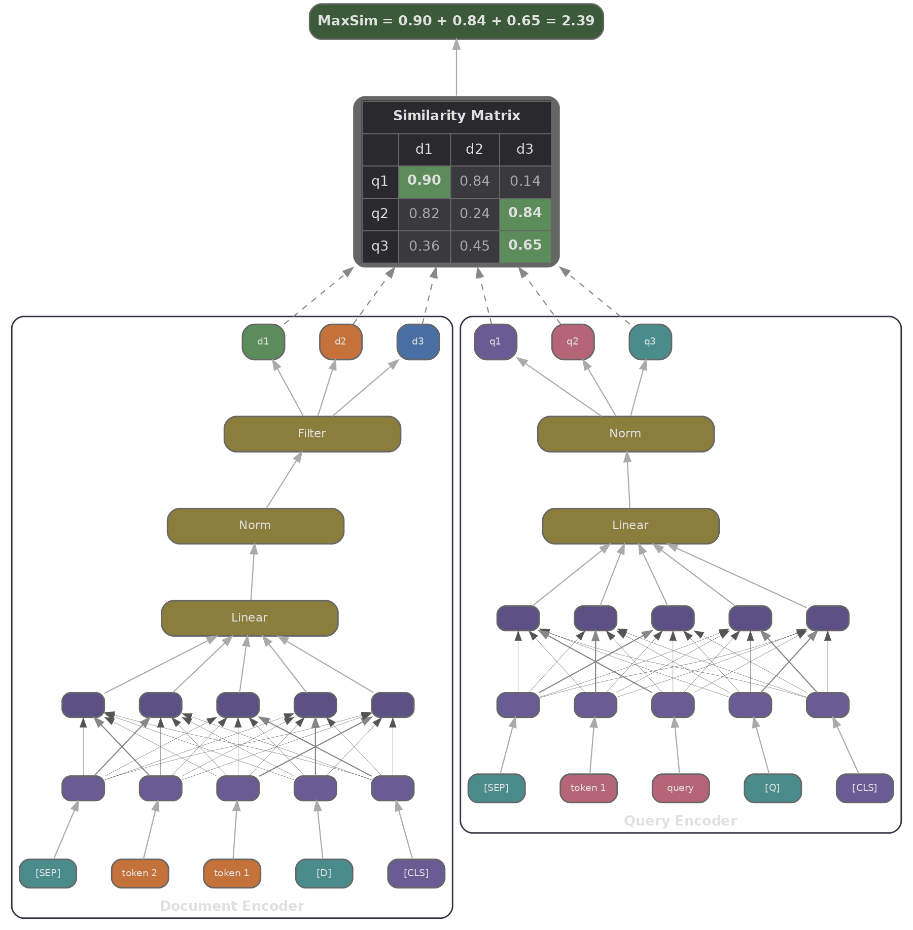
ColBERT encodes a query into a matrix $\mathbf{Q} \in \mathbb{R}^{N_q \times d}$ (one $d$-dimensional vector per query token) and a document into $\mathbf{D} \in \mathbb{R}^{N_d \times d}$ (one vector per document token). The scoring function, called MaxSim, works in two steps: for each query token $i$, we find the document token $j$ it is most similar to and take that similarity, then we sum the result over all query tokens.

This is a soft, differentiable form of term matching. A query token for "cardiac" will find its best match among the document's token vectors, whether that token corresponds to "cardiac", "heart", or even "coronary" (if those concepts happen to overlap in embedding space). The sum over query tokens means every part of the query contributes to the final score, weighted by how well the document addresses it.

In PyTorch, we can compute MaxSim across a batch of queries and passages with a single einsum followed by a max and a sum.

import torch

# q_reps: (num_queries, num_query_tokens, dim)
# p_reps: (num_passages, num_passage_tokens, dim)

# Step 1: compute all token-to-token dot products
# token_scores[q, p, i, j] = dot(q_reps[q, i], p_reps[p, j])
token_scores = torch.einsum('qin,pjn->qipj', q_reps, p_reps)

# Step 2: for each query token i, find the max over passage tokens j
# max_scores[q, p, i] = max_j token_scores[q, p, i, j]
max_scores, _ = token_scores.max(dim=-1)

# Step 3: sum over query tokens
# scores[q, p] = sum_i max_scores[q, p, i]
scores = max_scores.sum(dim=-1)

The einsum notation 'qin,pjn->qipj' says: for every combination of query $q$, passage $p$, query token $i$, and passage token $j$, compute the dot product over the embedding dimension $n$. The result is a 4D tensor with one similarity score per query-passage-token-token combination; the subsequent max and sum collapse those last two dimensions down to a single score per query-passage pair.

Compared to bi-encoder scoring, ColBERT's compute cost at query time is higher because MaxSim has to compare $N_q \times N_d$ token pairs per query-passage pair. But it is still far cheaper than a cross-encoder, since the document token matrices $\mathbf{D}$ are precomputed and cached.

How Does ColBERT Handle the 30× Index Blow-up?

ColBERT uses a contrastive training objective similar to DPR, but the loss operates on MaxSim scores rather than dot products of pooled vectors. During training, query representations are padded with [MASK] tokens to a fixed length, and these [MASK] embeddings learn to act as expansion slots (soft query terms that the model fills with relevant context). The effect is similar to SPLADE's vocabulary expansion from article 2, but it happens at the token embedding level rather than the vocabulary level.

The 30× index blow-up is a real deployment problem. The practical solution is a two-stage approach: approximate nearest-neighbour search over individual token vectors first identifies candidate passages (using a FAISS index over all document token vectors), and then we compute exact MaxSim scores for only those candidates.

ColBERTv2 (Santhanam et al., 2021) tackled the index size directly by introducing residual compression, which quantises document token vectors to 2-bit codes and reduces index size by 4-8× with minimal quality loss. PLAID (Santhanam et al., 2022) went further with centroid-based candidate generation: all document token vectors are clustered into $k$ centroids, and at query time each query token's nearest centroids determine which documents are scored. According to the PLAID paper, this reduces MaxSim computation by 50-100× while retaining top-10 retrieval quality.

Can One Model Produce All Three Retrieval Signals?

At this point in the track, we have seen three retrieval approaches: sparse (BM25/SPLADE), dense (bi-encoders), and late interaction (ColBERT). Each has strengths the others lack. Sparse retrieval is precise on rare keywords but misses paraphrases; dense retrieval handles synonymy well but can lose exact terms; late interaction offers the best quality but at the highest cost. A natural question is whether a single model can produce all three signals at once.

BGE-M3 (Chen et al., 2024) does exactly this. It is one encoder backbone with three output heads: a dense embedding (bi-encoder style), a sparse lexical weight vector (SPLADE style), and multi-vector representations for late interaction (ColBERT style). Each head fills a different gap.

• The head captures semantic similarity, handling paraphrase and synonymy well.
• The head does exact keyword matching, providing high precision for rare terms and technical jargon.
• The head performs fine-grained token matching with the highest quality, but also the highest cost.

In production, we can use dense retrieval as a fast first stage, sparse retrieval as a complementary signal fused via Reciprocal Rank Fusion (covered in article 5), and multi-vector scoring as a reranker on the top candidates. Because all three signals come from the same model, their representations are consistent with each other, avoiding the distribution mismatch that arises from mixing separate models.

BGE-M3's training has three stages, as described in Chen et al. (2024) : weakly supervised pretraining on 1.2 billion pairs from multilingual web data, fine-tuning on labelled retrieval data with all three loss heads simultaneously, and self-knowledge distillation. In the distillation step, the ensemble of all three scores serves as a soft teacher label for each individual head. The ensemble score tends to be more accurate than any single head, so distilling it back into each head encourages the three representations to stay mutually consistent.

The following chart illustrates (with simulated data) how these signals complement each other across different query types, and how combining them into a hybrid score tends to outperform any single signal.

import math, json
import js

# Simulate the complementary strengths of dense vs sparse vs multi-vector retrieval
# For a set of query types, show the relative recall@10

query_types = ["Semantic paraphrase", "Exact keyword", "Multi-hop reasoning", "Rare technical term", "Long question"]

# Simulated recall@10 values (0-100) for each retrieval type
dense_recall    = [92, 58, 75, 45, 83]
sparse_recall   = [54, 94, 60, 91, 49]
multivec_recall = [88, 85, 87, 83, 90]
hybrid_recall   = [95, 96, 91, 93, 93]

plot_data = [
    {
        "title": "Retrieval Signal Complementarity (Simulated Recall@10)",
        "x_label": "Query Type",
        "y_label": "Recall@10 (%)",
        "x_data": query_types,
        "lines": [
            {"label": "Dense",       "data": dense_recall,    "color": "#3b82f6"},
            {"label": "Sparse",      "data": sparse_recall,   "color": "#f59e0b"},
            {"label": "Multi-vector","data": multivec_recall,  "color": "#a855f7"},
            {"label": "Hybrid",      "data": hybrid_recall,   "color": "#10b981"},
        ]
    }
]
js.window.py_plot_data = json.dumps(plot_data)

Quiz

Test your understanding of late interaction and multi-vector retrieval.