Indexing and Chunking: Structuring Your Knowledge Base

The Chunking Problem

We've covered how to score documents (BM25, bi-encoders, ColBERT, rerankers) and how to combine scores (hybrid fusion). But all of these assume the documents are already in the index, ready to search. How do they get there? A RAG system needs to retrieve the specific passage that answers a query, not a 50-page PDF. Every document must be split into chunks before embedding, and then those embeddings need to be organised for fast lookup.

Small chunks (64–128 tokens) give precise retrieval but may lose context. A sentence about "the patient's condition" can lose critical context without the surrounding paragraph. Large chunks (512–1024 tokens) preserve context but dilute the embedding (a 1000-token chunk that is 80% boilerplate might embed similarly to many other chunks, harming precision).

Several chunking strategies exist, ranging from simple to fairly sophisticated.

• splits every $N$ tokens with an overlap of $M$ tokens (e.g. 512 tokens, 64 overlap). It is simple, fast, and robust, because the overlap prevents cutting a relevant sentence exactly at a chunk boundary.
• splits on sentences (using spaCy, NLTK, or regex) and groups them into chunks that stay under a token limit, preserving linguistic units.
• attempts to split on paragraphs first, then sentences, then words (whichever keeps chunks under the target size). LangChain's default text splitter uses this approach.
• embeds each sentence, computes cosine similarity between adjacent sentences, and splits where similarity drops below a threshold, grouping topically coherent text together.
• uses document structure (Markdown headers, HTML tags, PDF section breaks) to respect logical boundaries. A section titled "Related Work" is a natural chunk.

Chunk overlap matters because without it, a sentence that spans a chunk boundary will have its meaning cut in half. A 10-15% overlap (e.g. 64 tokens on a 512-token chunk) is a reasonable default.

HNSW: Approximate Nearest Neighbours

Once the chunks are embedded, we need to find the top-$k$ most similar vectors to a query vector efficiently. Exact nearest-neighbour search over $N$ vectors of dimension $d$ requires $O(Nd)$ operations per query. For 10 million 768-dimensional vectors, that is 7.68 billion multiplications per query, which is far too slow for interactive use.

Hierarchical Navigable Small World (HNSW) (Malkov & Yashunin, 2018) is the dominant approximate nearest-neighbour algorithm for dense retrieval. It builds a multi-layer graph where each node is a vector, and the layers form a hierarchy from coarse to fine.

• The contain few nodes with sparse, long-range connections, used for coarse navigation that quickly jumps to the region of the space containing the nearest neighbours.
• The contain all nodes with dense, local connections, used for fine-grained search that walks the local neighbourhood to find the actual nearest neighbours.

Three hyperparameters control the recall-speed trade-off.

• (connectivity) is the number of edges per node per layer. Higher $M$ gives better recall but uses more memory and slows construction; the default is typically 16.
• is the size of the dynamic candidate list during index construction. Larger values produce a better-quality index at the cost of a slower build; the default is typically 200.
• (efSearch) is the size of the candidate list during search. Larger values improve recall but slow queries; the default is typically 50. Unlike the other two, we can tune this per query without rebuilding the index.

HNSW search complexity is approximately $O(\log N)$ per query (traversing the hierarchy), compared to $O(N)$ for exact search. Empirical benchmarks on the ann-benchmarks suite show HNSW routinely reaching 95-99% recall@10 at 10-100x the speed of exact search, depending on index configuration and dataset. The fundamental trade-off is that increasing ef gives higher recall at the cost of slower queries.

HNSW is the default index in FAISS (`IndexHNSWFlat`), Weaviate, and Qdrant. One limitation is that HNSW graphs live entirely in memory. For 10 million 768-dimensional float32 vectors, the raw storage alone is $10^7 \times 768 \times 4 \text{ bytes} = 30.72\text{ GB}$, and the graph edges add further overhead on top of that. This makes HNSW considerably more memory-intensive than IVF-based indices.

IVF and Product Quantisation

Inverted File Index (IVF) takes a different approach: it first clusters all vectors into $C$ centroids using k-means (typically $C = 4\sqrt{N}$), then at query time searches only within the $n_{\text{probe}}$ nearest clusters. This reduces the search space from $N$ to roughly $\frac{N \cdot n_{\text{probe}}}{C}$ vectors.

FAISS `IndexIVFFlat` is the direct implementation. With $C=1024$ and $n_{\text{probe}}=8$, we search 8/1024 = 0.8% of the corpus per query. The trade-off is that recall depends on whether the nearest neighbours actually fall within the probed clusters. IVF tends to be faster than HNSW for very large $N$ (because it limits search to a fixed fraction of clusters, while HNSW's graph traversal overhead grows with corpus size), but it usually has lower recall at the same speed budget.

Product Quantisation (PQ) addresses the memory problem. Each 768-dimensional vector is split into $M$ subvectors of dimension $d/M = 768/M$, and each subvector is quantised to one of $K'=256$ codewords (stored as a 1-byte index). The original float32 vector (768 × 4 = 3072 bytes) is compressed to just $M$ bytes (a compression ratio of 3072/$M$).

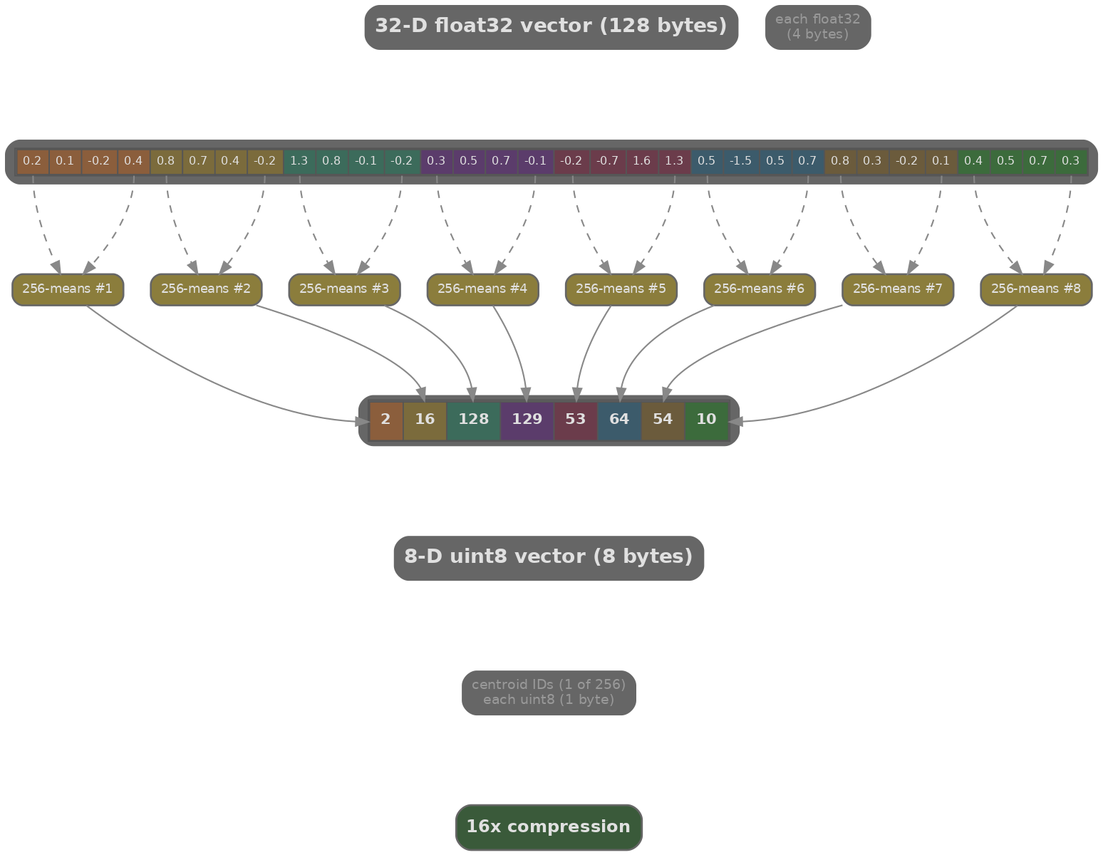
With $M=96$, a 768-dim vector compresses from 3072 bytes to 96 bytes (32× compression). The dot product between the query and a compressed vector is approximated as the sum of precomputed distance table lookups, one per subvector. This makes PQ not just memory-efficient but fast: the precomputed tables turn floating-point multiplications into integer look-ups.

IVFPQ combines both ideas: IVF partitioning limits the search scope, and PQ within each cluster compresses the stored vectors. FAISS `IndexIVFPQ` is the standard production choice for very large corpora (hundreds of millions of vectors), where the full cost per query is $n_{\text{probe}}$ cluster probes times the number of vectors per cluster times $M$ PQ look-ups per vector.

The simulation below illustrates how HNSW and IVF each trade recall for speed as we vary their search-time hyperparameters (ef for HNSW, nprobe for IVF).

import math, json
import js

# Simulate the recall vs speed trade-off for HNSW and IVF
# as a function of their search-time hyperparameters

# HNSW: increasing ef improves recall but increases latency
ef_values = [10, 20, 50, 100, 200, 500]
# Simulated: recall saturates near 1.0, latency grows linearly
hnsw_recall  = [round(1 - 0.12 * math.exp(-0.012 * ef), 3) for ef in ef_values]
hnsw_latency = [round(0.5 + 0.004 * ef, 2) for ef in ef_values]  # ms

# IVF: increasing nprobe improves recall but increases latency
nprobe_values = [1, 4, 8, 16, 32, 64]
ivf_recall  = [round(1 - 0.35 * math.exp(-0.06 * np), 3) for np in nprobe_values]
ivf_latency = [round(0.3 + 0.15 * np, 2) for np in nprobe_values]  # ms

# Common x-axis: latency in ms; plot recall vs latency
plot_data = [
    {
        "title": "Recall vs Query Latency: HNSW (ef) vs IVF (nprobe)",
        "x_label": "Query Latency (ms)",
        "y_label": "Recall@10",
        "x_data": [str(l) for l in hnsw_latency],
        "lines": [
            {"label": "HNSW (ef)",    "data": hnsw_recall,  "color": "#3b82f6"},
            {"label": "IVF (nprobe)", "data": ivf_recall,   "color": "#f59e0b"},
        ]
    }
]
js.window.py_plot_data = json.dumps(plot_data)

Quiz

Test your understanding of chunking strategies and vector indexing.