The Encoder

How Do We Assemble the Blocks?

We now have every piece we need: self-attention to let tokens talk to each other, multi-head attention to capture different relationship types in parallel, positional encoding to inject order, residual connections to keep gradients flowing, layer normalisation to stabilise training, and a feed-forward network to add per-token nonlinearity. The question is how these pieces fit together into a single coherent architecture, and the answer turns out to be surprisingly uniform.

An encoder layer chains the blocks in a fixed order: multi-head self-attention, then add-and-norm (a residual connection followed by layer norm), then the feed-forward network, then another add-and-norm. We stack $N$ of these identical layers on top of each other (the original transformer in Vaswani et al. (2017) used $N = 6$; BERT-base uses $N = 12$), and the output of the final layer is a sequence of contextual vectors, one per input token, where each vector has been refined through $N$ rounds of self-attention and nonlinear transformation.

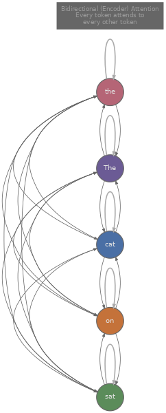
One detail distinguishes the encoder from the decoder we will build in the next article: the encoder uses bidirectional self-attention, meaning every token can attend to every other token in the sequence. There is no causal mask. When we compute attention for position $i$, the attention weights span all positions $1, 2, \ldots, n$, not just $1, \ldots, i$. This bidirectionality is precisely what makes encoders powerful for understanding tasks, because a token's representation can incorporate information from both its left and right context simultaneously.

We can see the full encoder layer in a compact PyTorch module. The following code stacks $N$ encoder layers and runs a dummy input through them.

import torch
import torch.nn as nn

class EncoderLayer(nn.Module):
    def __init__(self, d_model=768, n_heads=12, d_ff=3072, dropout=0.1):
        super().__init__()
        self.self_attn = nn.MultiheadAttention(d_model, n_heads, batch_first=True)
        self.ff = nn.Sequential(
            nn.Linear(d_model, d_ff),
            nn.GELU(),
            nn.Linear(d_ff, d_model),
        )
        self.norm1 = nn.LayerNorm(d_model)
        self.norm2 = nn.LayerNorm(d_model)
        self.drop  = nn.Dropout(dropout)

    def forward(self, x):
        # Multi-head self-attention + add & norm
        attn_out, _ = self.self_attn(x, x, x)       # Q, K, V all come from x
        x = self.norm1(x + self.drop(attn_out))      # residual + layer norm
        # Feed-forward + add & norm
        ff_out = self.ff(x)
        x = self.norm2(x + self.drop(ff_out))         # residual + layer norm
        return x

class TransformerEncoder(nn.Module):
    def __init__(self, n_layers=12, d_model=768, n_heads=12, d_ff=3072):
        super().__init__()
        self.layers = nn.ModuleList([
            EncoderLayer(d_model, n_heads, d_ff) for _ in range(n_layers)
        ])

    def forward(self, x):
        for layer in self.layers:
            x = layer(x)
        return x

# Quick shape check: batch=2, seq_len=16, d_model=768
encoder = TransformerEncoder(n_layers=6)
dummy = torch.randn(2, 16, 768)
out = encoder(dummy)
print(f"Input shape:  {dummy.shape}")   # [2, 16, 768]
print(f"Output shape: {out.shape}")     # [2, 16, 768]  — same shape, richer representations

Notice that the input and output shapes are identical. The encoder does not change the sequence length or dimension; it refines each token's representation in place. Every token's vector at the output carries information about the full input sequence, because each layer of bidirectional attention allows every position to mix information with every other position.

Why Mask Tokens Instead of Predicting the Next One?

Stacking encoder layers gives us an architecture, but we need a training objective that forces the model to learn useful representations. The most influential encoder model, BERT (Devlin et al., 2018) , introduced Masked Language Modelling (MLM) : randomly mask 15% of the input tokens and train the model to predict them from the surrounding context. This is fundamentally different from the left-to-right next-token prediction used in decoders, and the difference matters.

Consider the sentence "The cat sat on the [MASK]". To predict the masked word, the model needs to consider "The cat sat on the" from the left, but also anything that might follow from the right, such as "... and purred" or "... while it rained". If the model could only look left (as in a causal decoder), it would never see the right-side context that often disambiguates the answer. MLM forces bidirectional understanding because the masked token could appear anywhere in the sequence, and the context on both sides matters for predicting it accurately.

The 15% masking rate is itself a design choice. Devlin et al. found that masking too few tokens makes training inefficient (the model barely has to work on each example), while masking too many tokens removes so much context that accurate prediction becomes nearly impossible. Within that 15%, BERT applies a further split: 80% of the selected tokens are replaced with [MASK], 10% are replaced with a random token, and 10% are left unchanged. The random replacement and unchanged subsets exist to prevent the model from learning to ignore non-[MASK] tokens during fine-tuning (where no [MASK] tokens ever appear), though later work like RoBERTa (Liu et al., 2019) found that the exact split matters less than other training choices like batch size and data volume.

BERT was originally trained with a second objective called Next Sentence Prediction (NSP) : given two segments A and B, predict whether B actually follows A in the original document or was sampled randomly. The idea was that NSP would teach the model about inter-sentence coherence, which is useful for tasks like question answering where the relationship between two passages matters. In practice, however, RoBERTa showed that removing NSP either maintained or improved downstream performance, likely because the signal NSP provides is too easy (random sentence pairs are trivially distinguishable) and the task introduces noise that interferes with MLM learning. Most modern encoder models train with MLM only.

How Do We Use an Encoder for Downstream Tasks?

Once pre-training is done, we have a model that produces rich contextual representations for any input text, but those representations aren't directly answers to questions or labels for classification. We need to adapt them to specific tasks, and BERT's design includes a mechanism for this: the [CLS] token.

Every BERT input starts with a special [CLS] token prepended to the sequence. After passing through all $N$ encoder layers, the [CLS] position's output vector has attended to every token in the sequence across every layer, which makes it a natural candidate for a fixed-size sentence-level representation. For classification tasks (sentiment analysis, natural language inference, spam detection), we take the [CLS] vector and pass it through a small linear layer that maps it to the number of classes, then train with cross-entropy loss. This is the standard fine-tuning recipe: keep all the pre-trained encoder weights, add a task-specific head on top, and train the entire model end-to-end on labelled data for the target task.

For token-level tasks like Named Entity Recognition (NER), we use the output vector at each token position rather than just [CLS]. Each token's contextual vector is fed to a per-token classifier that predicts labels like PERSON, ORGANIZATION, LOCATION, or O (outside any entity). Because every token has attended to every other token through bidirectional attention, the model can use the full sentence context to decide whether "Washington" refers to a person, a city, or a state.

The fine-tuning code for classification is compact. We add a single linear layer on top of the pre-trained encoder and train on task-specific data.

import torch.nn as nn

class BertClassifier(nn.Module):
    def __init__(self, encoder, d_model=768, n_classes=2):
        super().__init__()
        self.encoder = encoder            # pre-trained transformer encoder
        self.classifier = nn.Linear(d_model, n_classes)

    def forward(self, x):
        hidden = self.encoder(x)          # (batch, seq_len, d_model)
        cls_vector = hidden[:, 0, :]      # take [CLS] position (index 0)
        return self.classifier(cls_vector) # (batch, n_classes)

# For NER, we'd classify every token position instead:
class BertNER(nn.Module):
    def __init__(self, encoder, d_model=768, n_labels=5):
        super().__init__()
        self.encoder = encoder
        self.token_classifier = nn.Linear(d_model, n_labels)

    def forward(self, x):
        hidden = self.encoder(x)          # (batch, seq_len, d_model)
        return self.token_classifier(hidden) # (batch, seq_len, n_labels)

This pattern (pre-train on a large unlabelled corpus, then fine-tune on a small labelled dataset) became the dominant paradigm in NLP from 2018 to roughly 2022, because the encoder's pre-trained representations capture so much linguistic knowledge that even a few hundred labelled examples are often enough for strong task performance.

When Should We Reach for an Encoder?

Encoder models tend to shine on tasks where we need to understand input text rather than generate new text. Classification, NER, semantic textual similarity, extractive question answering (highlighting a span in a passage), and sentence embedding for retrieval are all tasks where bidirectional context helps because the model can look at the entire input before making a decision. Encoder-based models like BERT, RoBERTa, and their descendants still tend to outperform decoder-only models of comparable size on these tasks, because bidirectional attention allows every token to gather signal from both directions in every layer, while a causal decoder can only condition on the left context.

The tradeoff is that encoders are not naturally suited for generation. An encoder processes the full input in one pass and produces a fixed-length representation, but it has no mechanism for producing tokens one at a time in a left-to-right fashion. Generating text requires the autoregressive structure we will see in the decoder (article 7), where each new token is conditioned on all previously generated tokens.

In practice, this division has become less rigid. Large decoder-only models like GPT-4 can classify text, extract entities, and compute similarity scores via prompting, often matching or exceeding BERT-class models on benchmarks. But for latency-sensitive production systems where a 110M-parameter BERT can run in a few milliseconds on a CPU, encoder models remain a practical and efficient choice. The question is usually not which architecture is more capable in the abstract, but which gives the best accuracy-latency-cost tradeoff for a specific deployment.

Quiz

Test your understanding of the transformer encoder and BERT.