The Decoder

From Understanding to Generation

The encoder we built in the previous article is powerful for understanding text, but it cannot generate new text. It takes a sequence in and produces a sequence of the same length out, with each position enriched by bidirectional context. If we ask it to continue a sentence, it has no mechanism for producing one token at a time, conditioning each new token on the ones that came before.

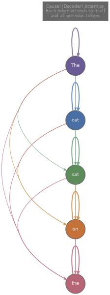
Generation requires a different structure. We need a model that, given tokens $x_1, x_2, \ldots, x_t$, predicts the probability distribution over the next token $x_{t+1}$, samples or selects from that distribution, appends the result, and repeats. This is autoregressive generation , and the architecture that supports it is the decoder . The decoder uses the same building blocks as the encoder (multi-head attention, add-and-norm, feed-forward network), but with one critical change: the self-attention is causal . A token at position $t$ can attend only to positions $1, 2, \ldots, t$, never to future positions. This is the causal mask we built in article 3, and it ensures that the model's prediction for position $t+1$ depends only on information that would actually be available at generation time.

The canonical decoder-only model is GPT (Radford et al., 2018) , which demonstrated that a transformer decoder trained on a large corpus with a simple next-token prediction objective could then be fine-tuned for a wide range of downstream tasks. The training objective is straightforward: given a sequence of tokens, maximise the log-probability of each token conditioned on the preceding tokens.

Each term in this sum asks the model to assign high probability to the token that actually comes next. If the model is confident and correct, $P(x_t \mid \ldots)$ is close to 1 and $-\log P$ is close to 0. If the model is surprised by the actual next token, $P(x_t \mid \ldots)$ is small and the loss is large. Averaging over all $T$ positions in the sequence means every position contributes a training signal, which makes the objective highly data-efficient compared to MLM (where only 15% of positions produce a loss).

During training, we can compute the loss for all positions in parallel using the causal mask. The model processes the entire sequence at once, the mask ensures position $t$ only sees positions $\leq t$, and we compute the loss at every position simultaneously. This is called teacher forcing : we feed the ground-truth tokens at every position rather than the model's own predictions, which avoids error accumulation and allows efficient batched computation. At inference time, however, we must generate one token at a time, feed it back in, and repeat.

How Do We Choose the Next Token?

Once the model produces a probability distribution over the vocabulary for position $t+1$, we need a strategy for picking which token to actually emit. This choice matters more than it might seem: the same model can produce repetitive, boring text or creative, diverse text depending entirely on the sampling strategy.

The simplest approach is greedy decoding : always pick the token with the highest probability. This is fast (no randomness to manage) and deterministic (the same prompt always produces the same output), but it tends to produce repetitive, generic text. Because the highest-probability token at each step is usually a common, safe word, greedy decoding often falls into loops or produces bland output that never takes risks.

We can implement greedy decoding and the sampling alternatives in a few lines each. The code below shows all four strategies operating on the same logit vector.

import math
import random

random.seed(42)

# Simulated raw logits for a vocabulary of 8 tokens
vocab = ["the", "cat", "sat", "on", "a", "dog", "mat", "hat"]
logits = [2.0, 1.5, 0.8, 0.3, 0.1, 1.2, 0.6, 0.9]

def softmax(logits):
    m = max(logits)
    exps = [math.exp(x - m) for x in logits]
    s = sum(exps)
    return [e / s for e in exps]

# 1. Greedy: pick the highest-probability token
probs = softmax(logits)
greedy_idx = probs.index(max(probs))
print(f"Greedy: '{vocab[greedy_idx]}' (p={probs[greedy_idx]:.3f})")

# 2. Temperature: scale logits before softmax
def sample_with_temperature(logits, T):
    scaled = [l / T for l in logits]
    probs = softmax(scaled)
    r = random.random()
    cumulative = 0.0
    for i, p in enumerate(probs):
        cumulative += p
        if r < cumulative:
            return i, probs
    return len(probs) - 1, probs

idx_low, p_low = sample_with_temperature(logits, T=0.3)
idx_high, p_high = sample_with_temperature(logits, T=2.0)
print(f"Temp=0.3: '{vocab[idx_low]}'  (top prob={max(p_low):.3f}, nearly greedy)")
print(f"Temp=2.0: '{vocab[idx_high]}' (top prob={max(p_high):.3f}, very spread out)")

# 3. Top-k: sample from the k most probable tokens
def sample_top_k(logits, k):
    indexed = sorted(enumerate(logits), key=lambda x: -x[1])[:k]
    top_logits = [l for _, l in indexed]
    top_indices = [i for i, _ in indexed]
    probs = softmax(top_logits)
    r = random.random()
    cumulative = 0.0
    for i, p in enumerate(probs):
        cumulative += p
        if r < cumulative:
            return top_indices[i], probs, top_indices
    return top_indices[-1], probs, top_indices

idx_k, probs_k, kept_k = sample_top_k(logits, k=3)
print(f"Top-k=3:  '{vocab[idx_k]}'  (candidates: {[vocab[i] for i in kept_k]})")

# 4. Top-p (nucleus): sample from smallest set with cumulative prob >= p
def sample_top_p(logits, p_threshold):
    probs = softmax(logits)
    indexed = sorted(enumerate(probs), key=lambda x: -x[1])
    cumulative = 0.0
    nucleus = []
    for i, p in indexed:
        cumulative += p
        nucleus.append((i, p))
        if cumulative >= p_threshold:
            break
    # Re-normalise within the nucleus
    total = sum(p for _, p in nucleus)
    r = random.random()
    cumulative = 0.0
    for i, p in nucleus:
        cumulative += p / total
        if r < cumulative:
            return i, [vocab[idx] for idx, _ in nucleus]
    return nucleus[-1][0], [vocab[idx] for idx, _ in nucleus]

idx_p, nucleus_tokens = sample_top_p(logits, p_threshold=0.8)
print(f"Top-p=0.8: '{vocab[idx_p]}' (nucleus: {nucleus_tokens})")

Let us walk through what each strategy actually does to the distribution.

Temperature divides every logit by a scalar $T$ before softmax. When $T \to 0$, the division amplifies differences between logits so much that the largest logit dominates completely, recovering greedy decoding in the limit. When $T \to \infty$, all logits become $\approx 0$ after division, and softmax produces a nearly uniform distribution, so the model samples almost randomly. In practice, values between 0.7 and 1.0 are common for coherent generation, while values above 1.0 encourage creativity at the cost of occasional nonsense.

Top-k sampling (Fan et al., 2018) restricts the candidate set to the $k$ tokens with the highest probabilities, zeroes out everything else, and re-normalises. This prevents the model from ever sampling extremely low-probability tokens (which tend to be incoherent), but the fixed $k$ is a weakness: when the model is confident, even $k = 10$ might include junk tokens that dilute quality; when the distribution is flat and the model is genuinely uncertain, $k = 10$ might exclude perfectly reasonable continuations.

Nucleus sampling (top-p) (Holtzman et al., 2019) solves this by adapting the candidate set size dynamically. Instead of fixing $k$, we sort tokens by descending probability and keep adding tokens to the nucleus until their cumulative probability reaches a threshold $p$ (commonly 0.9 or 0.95). When the model is confident, the nucleus might contain just 2 or 3 tokens; when uncertain, it might contain hundreds. This adaptivity tends to produce more natural text than fixed top-k, and nucleus sampling has become the default strategy in most production language model APIs.

How Do We Know If the Model Is Good?

We have a model that generates text and a set of strategies for choosing tokens. But how do we quantify whether the model itself (independent of the sampling strategy) has learned the language well? The standard metric for language models is perplexity , which measures how surprised the model is by a held-out test set.

Perplexity is defined as the exponential of the average negative log-likelihood:

The expression inside the exponential is exactly the cross-entropy loss we train with, so perplexity is $e^{\text{loss}}$. This transformation from log-space back to probability-space gives perplexity a direct interpretation: a perplexity of $k$ means the model is, on average, as uncertain as if it were choosing uniformly among $k$ options at each step. If a model achieves perplexity 20 on a test set, it is as surprised as if it had to pick from 20 equally likely tokens at every position.

To see why lower is better, consider the extremes. If the model assigns probability 1.0 to the correct token at every position (a perfect model), the loss is $0$ and perplexity is $e^0 = 1$. If the model assigns equal probability $1/V$ to every token in a vocabulary of size $V$ (a model that has learned nothing), the loss is $\log V$ and perplexity is $V$, which for GPT-2's vocabulary is around 50,257. Real models fall between these bounds, and improvements from 25 to 20 perplexity typically correspond to noticeably better generation quality.

We can compute perplexity from a set of per-token probabilities. The code below simulates a short sequence and walks through the calculation.

import math

# Simulated model probabilities for each token in a 10-token sequence
# Higher values = model was more confident about the correct token
token_probs = [0.85, 0.72, 0.30, 0.95, 0.60, 0.45, 0.88, 0.15, 0.70, 0.55]
tokens      = ["The", "cat",  "sat", "on", "the", "old",  "mat", "and", "then", "left"]

# Per-token loss and perplexity
total_nll = 0.0
print("Token-level breakdown:")
for i, (tok, p) in enumerate(zip(tokens, token_probs)):
    nll = -math.log(p)
    total_nll += nll
    print(f"  '{tok}':  P={p:.2f}  ->  -log P = {nll:.3f}")

avg_nll = total_nll / len(tokens)
ppl = math.exp(avg_nll)

print(f"\nAverage NLL (cross-entropy loss): {avg_nll:.4f}")
print(f"Perplexity = exp({avg_nll:.4f}) = {ppl:.2f}")
print(f"\nInterpretation: the model is as uncertain as choosing")
print(f"uniformly among ~{ppl:.0f} tokens at each step.")

Notice how the token "and" (with $P = 0.15$) contributes a much larger loss than "on" (with $P = 0.95$). Perplexity is dominated by the tokens the model finds most surprising, which is why rare words, proper nouns, and unexpected transitions tend to be the hardest parts of a test set.

Beyond perplexity, language models are often evaluated on downstream benchmarks that test specific capabilities. HellaSwag (Zellers et al., 2019) tests common-sense reasoning by presenting a scenario and four possible continuations, asking the model to pick the most plausible one. MMLU (Hendrycks et al., 2020) covers 57 subjects from elementary math to professional law, measuring how much world knowledge the model has absorbed. These benchmarks complement perplexity because a model can have low perplexity (it predicts text well) while still failing at reasoning tasks that require combining knowledge across domains.

What Should Training Look Like?

Pre-training a decoder language model means running the next-token prediction objective over billions of tokens for many thousands of gradient steps. The loss curves during this process have a characteristic shape that is worth understanding, because recognising what healthy and unhealthy training looks like helps diagnose problems early.

Training loss starts high (the model is random, so its per-token predictions are nearly uniform across the vocabulary) and drops steeply in the first few thousand steps as the model learns basic syntax, common word frequencies, and short-range dependencies. The descent then gradually flattens as the model moves from easy patterns (predicting "the" after "in") to harder ones (predicting the correct name in "The 44th president of the United States was ___"). A typical GPT-2 scale training run might see training loss drop from ~10 to ~3 over the full run, corresponding to a perplexity reduction from ~22,000 to ~20.

Validation loss (computed on held-out data that the model never trains on) should track training loss closely during healthy training. The gap between them reveals generalisation: if training loss keeps decreasing but validation loss plateaus or increases, the model is memorising training data rather than learning generalisable patterns. This is overfitting, and it tends to happen when the model is too large for the amount of training data or when training runs for too many epochs.

Scaling laws (Kaplan et al., 2020) showed that validation loss follows power-law relationships with model size, dataset size, and compute budget: double the parameters and the loss drops by a predictable amount. Chinchilla (Hoffmann et al., 2022) refined this by showing that many models were undertrained (too many parameters, not enough data), and that the optimal ratio is roughly 20 tokens of training data per parameter. A 1B-parameter model should see about 20B tokens, and a 70B model should see about 1.4T tokens for compute-optimal training.

The following code simulates what healthy training and validation loss curves typically look like, alongside an overfitting scenario where the model is too large for the data.

import math, json
import js

steps = list(range(0, 5001, 100))

def healthy_train(s):
    return 3.5 * math.exp(-s / 800) + 2.8 + 0.15 * math.exp(-s / 3000)

def healthy_val(s):
    return 3.5 * math.exp(-s / 800) + 2.85 + 0.15 * math.exp(-s / 3000)

def overfit_train(s):
    return 3.5 * math.exp(-s / 600) + 2.5 + 0.2 * math.exp(-s / 2000)

def overfit_val(s):
    base = 3.5 * math.exp(-s / 800) + 2.9 + 0.15 * math.exp(-s / 3000)
    if s > 2000:
        base += 0.0002 * (s - 2000)
    return base

train_h = [round(healthy_train(s), 3) for s in steps]
val_h   = [round(healthy_val(s), 3) for s in steps]
train_o = [round(overfit_train(s), 3) for s in steps]
val_o   = [round(overfit_val(s), 3) for s in steps]

plot_data = [
    {
        "title": "Healthy Training (enough data)",
        "x_label": "Steps",
        "y_label": "Loss",
        "x_data": steps,
        "lines": [
            {"label": "Train loss", "data": train_h, "color": "#3b82f6"},
            {"label": "Val loss",   "data": val_h,   "color": "#ef4444"},
        ]
    },
    {
        "title": "Overfitting (too little data)",
        "x_label": "Steps",
        "y_label": "Loss",
        "x_data": steps,
        "lines": [
            {"label": "Train loss", "data": train_o, "color": "#3b82f6"},
            {"label": "Val loss",   "data": val_o,   "color": "#ef4444"},
        ]
    }
]
js.window.py_plot_data = json.dumps(plot_data)

In the healthy case, training and validation loss descend together and nearly converge, which means the model is learning patterns that generalise beyond the training set. In the overfitting case, training loss continues to drop (the model keeps memorising), but validation loss turns upward after step 2000, signalling that the model's predictions on unseen data are getting worse. In practice, this is why we monitor validation loss and stop training (or reduce the learning rate) when it stops improving.

Quiz

Test your understanding of the decoder, sampling strategies, and evaluation.