Causal Masking and the Attention Matrix

Why Can't a Decoder Look Ahead?

The previous article described attention as a mechanism where every position can attend to every other position. That works perfectly when we're encoding an input (like BERT processing a sentence for classification), because the entire input is available at once and every token benefits from seeing the full context in both directions. But when a model is generating text — predicting the next token given everything before it — we face a fundamental constraint: the model cannot see the future.

Consider a language model being trained on the sentence "the cat sat on the mat." At position 3, the model should predict "sat" from the context "the cat". If position 3 could attend to position 4 ("on"), position 5 ("the"), and position 6 ("mat"), the prediction task becomes trivial (the model just copies the answer instead of learning to predict it). During generation at inference time, positions 4, 5, and 6 don't even exist yet when we're producing position 3, so allowing attention to those positions during training would create a mismatch between training and inference conditions.

This is not just a practical concern about cheating on the training loss. It's architecturally necessary for autoregressive generation to work at all. When we generate token by token at inference time, each new token is produced conditioned only on previous tokens. If the model were trained with access to future tokens, the representations it learned would depend on information that simply isn't available during generation, and the model's outputs would be incoherent.

So we need a way to enforce the constraint that position $i$ can only attend to positions $j \leq i$. We could accomplish this by literally running attention $T$ separate times (once per position, each time only including the appropriate tokens), but that would destroy the parallelism that makes transformers fast. Instead, we use a causal mask (a single operation that blocks future positions while keeping the full computation parallelised).

How Does the Mask Actually Work?

Recall from the previous article that the raw attention scores form a $T \times T$ matrix $S = QK^\top / \sqrt{d_k}$, where $S_{ij}$ is the score between position $i$'s query and position $j$'s key. Before applying softmax, we add a mask matrix $M$ to these scores:

The mask $M \in \mathbb{R}^{T \times T}$ is defined as:

For a sequence of 4 tokens, the mask looks like this:

When we add $-\infty$ to a score and then take the softmax, the exponent $e^{-\infty} = 0$, so that position receives exactly zero attention weight. The allowed positions (where $M_{ij} = 0$) pass through unchanged. After softmax, each row still sums to 1, but the probability mass is distributed only over the current and earlier positions.

Let's consider what happens row by row. Row 1 (position 0, the first token) has $-\infty$ everywhere except column 0, so after softmax it becomes $[1, 0, 0, 0]$ (the first token can only attend to itself). Row 2 distributes its weight across columns 0 and 1. Row 3 distributes across columns 0, 1, and 2. Row 4 attends to all positions. Each successive position has access to strictly more context than the one before it.

The implementation is straightforward. We can build the mask as a lower-triangular matrix of ones, invert it, and multiply by a large negative number.

import numpy as np

T = 5  # sequence length

# Lower-triangular matrix: 1 where attention is allowed, 0 where blocked
causal = np.tril(np.ones((T, T)))
print("Causal matrix (1 = allowed, 0 = blocked):")
print(causal.astype(int))

# Convert to additive mask: 0 where allowed, -1e9 where blocked
mask = (1 - causal) * (-1e9)
print("\nAdditive mask (0 = pass through, -1e9 = block):")
print(mask)

# Simulate: random scores + mask + softmax
np.random.seed(7)
scores = np.random.randn(T, T)  # raw attention scores

def softmax(x):
    e = np.exp(x - x.max(axis=-1, keepdims=True))
    return e / e.sum(axis=-1, keepdims=True)

masked_scores = scores + mask
attn_weights = softmax(masked_scores)

print("\nAttention weights after causal masking:")
print(np.round(attn_weights, 4))
print("\nRow sums:", np.round(attn_weights.sum(axis=1), 6))
print("\nNote: each row attends only to positions <= its own index.")

In the output, notice how position 0 puts all its weight on itself (the only option), while position 4 spreads attention across all five positions. The upper-right triangle is exactly zero (no information leaks from the future).

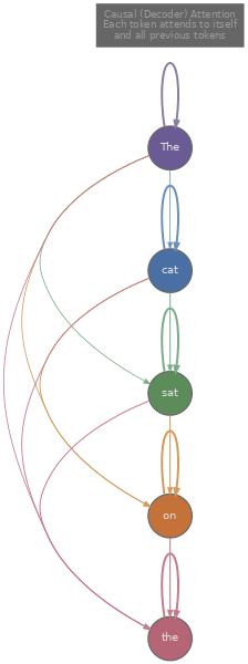
Thinking About Attention as a Graph

There's a way to think about the attention matrix that makes causal masking feel less like an arbitrary constraint and more like a natural structure: treat each token as a node in a directed graph , where an edge from node $j$ to node $i$ means "position $i$ attends to position $j$" (information flows from $j$ to $i$). The $T \times T$ attention weight matrix is exactly this graph's weighted adjacency matrix.

Without any masking (bidirectional attention, as in an encoder like BERT), the graph is fully connected: every node has edges to every other node, including itself. For $T = 4$ tokens, that's $4 \times 4 = 16$ directed edges. Every token can gather information from every other token, which is exactly what we want when the entire input is available and we're building contextual representations for downstream tasks like classification or named entity recognition.

With a causal mask, the graph is a lower-triangular adjacency matrix, and the connectivity builds up token by token. Token 0 has exactly one edge (a self-loop). Token 1 has two edges: to itself and to token 0. Token 2 has three edges: to tokens 0, 1, and 2. In general, token $i$ has exactly $i + 1$ edges. The total number of edges is $1 + 2 + 3 + \cdots + T = T(T+1)/2$, roughly half the edges of the fully connected case.

This graph perspective makes several things concrete. The amount of context available to a token increases linearly with its position: the first token is the most information-starved (it only sees itself), while the last token is the most information-rich (it sees everything). This asymmetry is inherent to autoregressive modelling, and it's one reason why the very first token's representation tends to be less useful than later tokens' in practice.

We can visualise this by building the graph for a small sequence and comparing the causal and bidirectional cases.

import numpy as np

tokens = ["The", "cat", "sat", "on"]
T = len(tokens)

# Bidirectional (encoder): full connectivity
print("=== Bidirectional (Encoder) Attention ===")
print(f"Adjacency matrix ({T}x{T}, all ones):")
bi_adj = np.ones((T, T), dtype=int)
print(bi_adj)
print(f"Total edges: {bi_adj.sum()}")
print()
for i, tok in enumerate(tokens):
    targets = [tokens[j] for j in range(T)]
    print(f"  '{tok}' (pos {i}) attends to: {targets}")

print()

# Causal (decoder): lower triangular
print("=== Causal (Decoder) Attention ===")
print(f"Adjacency matrix ({T}x{T}, lower triangular):")
causal_adj = np.tril(np.ones((T, T), dtype=int))
print(causal_adj)
print(f"Total edges: {causal_adj.sum()} (= T*(T+1)/2 = {T*(T+1)//2})")
print()
for i, tok in enumerate(tokens):
    targets = [tokens[j] for j in range(i + 1)]
    print(f"  '{tok}' (pos {i}) attends to: {targets}")

The output shows the structural difference clearly. In the bidirectional case, "The" at position 0 attends to all four tokens, including "on" at position 3. In the causal case, "The" attends only to itself, while "on" at position 3 attends to all preceding tokens including itself. The adjacency matrix transitions from a matrix of all ones to a lower-triangular matrix, and every intermediate structure (like attending to all tokens within a fixed window, or attending to every $k$-th token) corresponds to a different sparsity pattern in this same $T \times T$ matrix.

The graph framing also clarifies the computational cost. Each edge in the graph corresponds to one attention score computation (one dot product between a query and a key). Bidirectional attention computes $T^2$ scores, causal attention computes $T(T+1)/2 \approx T^2/2$ scores, and sparse attention patterns compute even fewer. The sparsity of the graph directly translates to computational savings, which is why efficient attention research (Tay et al., 2020) focuses heavily on finding good sparse structures that preserve model quality while reducing the $O(T^2)$ cost.

Putting It All Together: Masked Self-Attention in Practice

Let's now implement a complete masked self-attention forward pass that combines everything from this article and the previous one: query-key-value projections, scaled dot products, causal masking, and the weighted sum. This is the core computation inside every decoder layer of models like GPT-2, GPT-3, and LLaMA.

import numpy as np

np.random.seed(42)

def masked_self_attention(X, W_Q, W_K, W_V):
    """
    Single-head causal self-attention.
    X:   (T, d_model) input embeddings
    W_Q: (d_model, d_k) query projection
    W_K: (d_model, d_k) key projection
    W_V: (d_model, d_v) value projection
    """
    T = X.shape[0]
    d_k = W_Q.shape[1]

    # Step 1: Project to Q, K, V
    Q = X @ W_Q
    K = X @ W_K
    V = X @ W_V

    # Step 2: Scaled dot-product scores
    scores = (Q @ K.T) / np.sqrt(d_k)

    # Step 3: Apply causal mask
    mask = np.triu(np.ones((T, T)) * (-1e9), k=1)
    scores = scores + mask

    # Step 4: Softmax (row-wise)
    e = np.exp(scores - scores.max(axis=-1, keepdims=True))
    attn = e / e.sum(axis=-1, keepdims=True)

    # Step 5: Weighted sum of values
    output = attn @ V

    return output, attn

# Setup
T, d_model, d_k, d_v = 5, 16, 8, 8
X = np.random.randn(T, d_model)
W_Q = np.random.randn(d_model, d_k) * 0.1
W_K = np.random.randn(d_model, d_k) * 0.1
W_V = np.random.randn(d_model, d_v) * 0.1

output, attn = masked_self_attention(X, W_Q, W_K, W_V)

print("Attention weights (causal, T=5):")
print(np.round(attn, 3))
print(f"\nOutput shape: {output.shape}")
print(f"\nPosition 0 sees only itself:     weights = {np.round(attn[0], 3)}")
print(f"Position 4 sees all 5 positions: weights = {np.round(attn[4], 3)}")

The output confirms what we expect: position 0 places all its weight (1.0) on itself, because the causal mask blocks every other position. Position 4, at the end of the sequence, distributes its attention across all five positions according to the learned query-key similarities. The upper triangle of the attention matrix is exactly zero.

It's worth noting that the mask itself has no learned parameters. It's a fixed structural constraint determined entirely by the sequence positions (the same binary pattern regardless of what the tokens are). All the learning happens in $W^Q$, $W^K$, and $W^V$, which determine how tokens interact within the allowed connections. The mask defines the graph topology; the projections define the edge weights.

We've now covered the three core components of transformer attention: the query-key-value framework (article 2), the scaled dot-product formula (article 2), and the causal mask (this article). Together, these form the self-attention sublayer that repeats in every transformer decoder block. The remaining components of a full transformer layer (multi-head attention, residual connections, layer normalisation, and feed-forward networks) build on this foundation, and we'll cover them as we move through the track.

Quiz

Test your understanding of causal masking and the attention matrix.